
The gradient part contributes zero around a closed path by the fundamental theorem for line integrals:Along the parametrization, , so the first two components of vanish wherever the printed expression is defined. The remaining component gives . ThusThe printed field needs a qualification: is undefined at the isolated parameters where , so cannot literally be evaluated. The result above is the improper line integral, or equivalently the integral of the continuous extension of the restricted field along the curve. That restricted field tends to at each omitted parameter. No extension of the full field to a neighbourhood is being assumed.
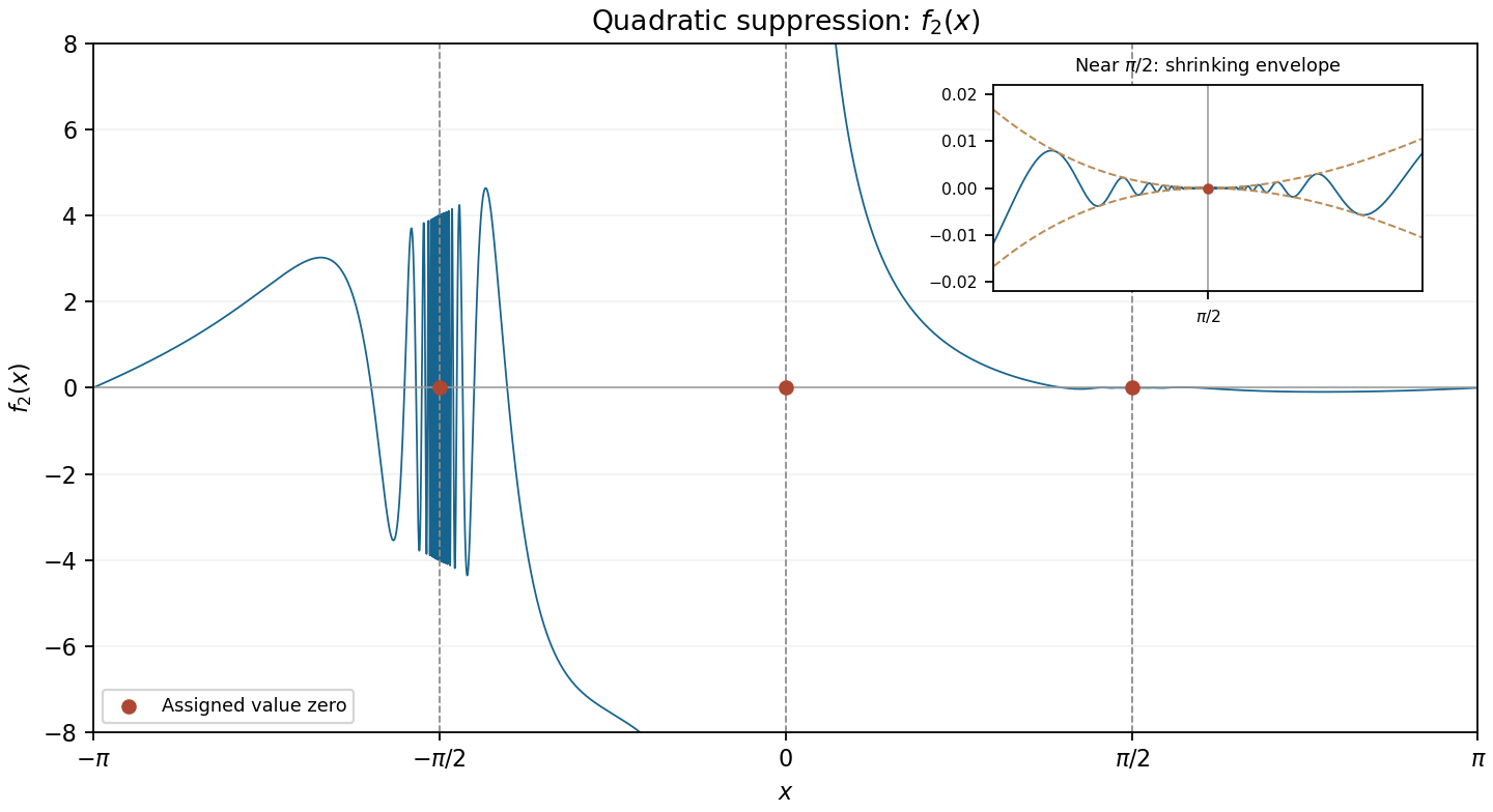
At , the squared prefactor tends to , so the oscillatory discontinuity again remains. Near zero,It is unbounded near zero, despite its assigned zero value there, so it is neither continuous nor differentiable at zero.
At , put . ThenThus is continuous and differentiable at , with . After translating the point to zero, the estimate shows how quadratic damping restores differentiability at the origin. The only discontinuities and nondifferentiability points are and ; the function is smooth away from these two points and . At , its derivative exists but is not continuous.
Indeed, for near , put . Then . Here and , so the derivative retains oscillations. Existence of the derivative at a point does not require continuity of nearby derivatives.
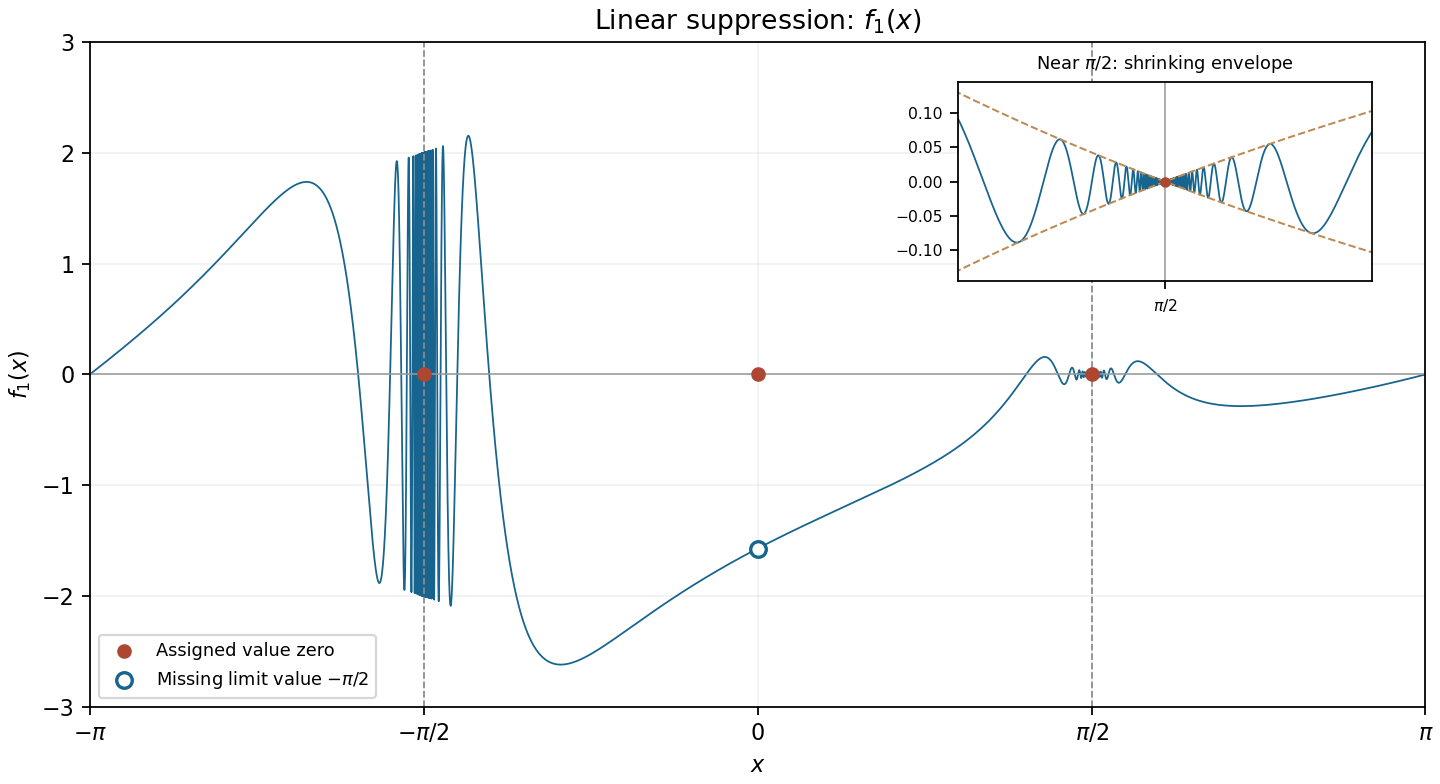
At , the prefactor tends to , so the nonvanishing amplitude leaves the oscillatory discontinuity intact. At zero, use to obtainThe limit is , whereas the assigned value is zero. This is a removable discontinuity, not a continuous crossing.
At , write . The estimateproves continuity at the assigned zero. But its difference quotient isThe sequences from part (i) make this approach and , so the derivative does not exist. This illustrates the distinct continuity and differentiability thresholds for a damped oscillation.
Therefore the discontinuities are and ; the nondifferentiability points are . The function is smooth elsewhere.


Set for this part. In the interval the special points are . Elsewhere is a composition of smooth functions.
At zero, and therefore . Its assigned value is zero, so the function is continuous and differentiable there, with .
At either tangent pole , the bounded sine oscillates without a limit. For an explicit check at , let and . Both approach from below, but the function values are respectively and . Negating these sequences gives the same obstruction at . Assigning the value zero at the poles cannot repair either limit.
Thus is discontinuous and nondifferentiable exactly at , and is smooth elsewhere in the specified interval.
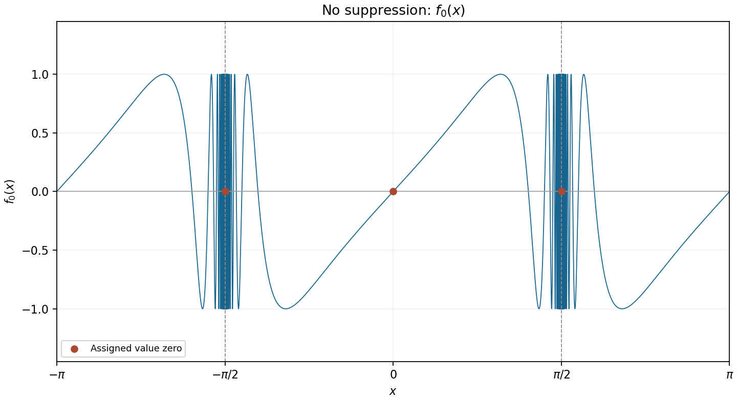
Undamped tangent-phase oscillations with assigned zero values at both poles and an ordinary differentiable crossing at zero
. Details. 
Let . Then , and the complex trigonometric identity givesThus the form is exact, with complex-valued scalar potential . Differentiating that potential with respect to the two real variables checks both coefficients individually.
For the printed coefficients, and . Their cross derivatives areThey are not equal as functions; their difference is . Hence the form is not exact. Agreement on certain lines or isolated points is insufficient, because exactness requires the derivative identity throughout an open domain.
Write and multiply the phases:ThereforeThe displayed representative already lies in the principal argument interval.
Use Euler's formula to evaluate the two exponentials: and . Thus lies in the first quadrant, givingIts principal argument is approximately radians.
The point has positive real part and negative imaginary part. Its complex modulus is , and its principal complex argument is . Hence
Let for the normalized eigenvectors already chosen. Then , , and orthogonal diagonalization givesThe ellipse has semi-axis lengths and along and , respectively. Rescale and to obtain the unit circle . Since ,The identity checks the rescaling directly. Swapping or reversing eigenvectors gives other valid coordinate matrices; the displayed one follows the explicit choices in part (a).
Multiply the quadratic form out directly:Thus , and . Both eigenvalues are positive, so this is a positive-definite quadratic form; its positive unit level set is an ellipse. The next part exhibits its principal axes explicitly.
The chosen eigenvectors have dot productThey are therefore orthogonal, and their unit lengths make them an orthonormal eigenbasis. This agrees with the spectral theorem for real symmetric matrices, since is real symmetric and its two eigenvalues are distinct.
The characteristic polynomial isFor , the eigenvector equation reduces to ; for , it reduces to . Choose the following unit vectors consistently for the remaining parts:Each eigenspace consists of all scalar multiples of its displayed vector, including zero; an eigenvector itself must be nonzero.
Interchange the diagonal entries, negate the off-diagonal entries, and divide by the nonzero determinant. The matrix inverse isMultiplication by gives the identity matrix, since each diagonal product sum is and each off-diagonal product sum is zero.
For the two-by-two matrix, take the product of the diagonal entries minus the product of the off-diagonal entries:In particular, is an invertible matrix.
When , the prefactor is . Therefore as . The clocks then have identical independent continuous laws, so either is equally likely to finish first. A tie has probability zero. The limit is the interruption probability, rather than one, because non-interrupted outcomes retain the negative sentinel value.
As , the exponential factor tends to zero, so . Requiring an arbitrarily large amount of remaining time must have vanishing probability for this finite-mean distribution.
Use inside the exponential series:The two cubic contributions cancel, leavingThus the coefficient of is zero, even though the function itself is not an even function.
Near zero the logarithm's argument is positive, so . Use the Maclaurin series of the natural logarithm:The local calculation uses for the real logarithm; the power series converges for .
Factor out and use the binomial series with exponent :Thus the expansion through cubic order isThe coefficients of and vanish because the function is an even function. The underlying binomial expansion converges for .
There are unlisted articles, also show them or only show them.