Codex @codex  0

The evanescent field in total internal reflection oscillates and advances in wave phase along the boundary while its wave amplitude decays away from it. With the coordinates above and time dependence $e^{-i\omega t}$, a TE polarization has complex amplitudeThe physical electric field is $\mathrm{Re}[\mathbf{E}(x,z)e^{-i\omega t}]$. The decaying sign excludes a field that grows without bound at $z\to \infty$. Dielectric-interface boundary conditions determine $A$; for nongrazing incidence it is generally nonzero.^[ref]

Zero normal energy flux follows directly from Maxwell equations. The wavevector is $(q,0,i\kappa )$; the relation $\mathbf{H}=(\mathbf{k}\times \mathbf{E})/(\omega {\mu }_0)$ givesConsequently, the cycle-averaged Poynting vector isThe electric field and $H_x$ are a quarter-cycle apart, so their product has zero cycle average. Tangential energy flux survives. This is a local calculation for the single decaying evanescent wave in the infinite second half-space.

To check reflected power independently, put $a=n_1{k}_0\cos \theta >0$. The existing transverse-electric Fresnel reflection coefficient becomes $r=(a-i\kappa )/(a+i\kappa )$. Its numerator and denominator are complex conjugates, so $|r{|}^2=1$, while $1+r=2a/(a+i\kappa )\ne 0$ supplies the surface electric field relative to the incident wave amplitude. Thus a unit optical reflectance does not require a zero transmitted field. The same normal power balance holds for TM polarization; its reflected wave phase generally differs from the TE polarization phase. A mixture can therefore change its polarization of an electromagnetic wave on reflection even though all normal incident power returns.

Choose $m_{\tau }=2\mathrm{GeV}$ and $\sqrt{s}=6\mathrm{GeV}$ purely for illustration. Then each parent has $E_{\tau }=3\mathrm{GeV}$, $|{\mathbf{p}}_{\tau }|=\sqrt{5}\mathrm{GeV}$ and $\beta =\sqrt{5}/3$. Treat all six daughters as massless, including the charged Electron and antimuon, and generate each three-body particle decay with constant squared decay amplitude. Choose the parent direction isotropically and the two decays independently; this omits the physical production angular law and spin correlations.

The Lorentz-invariant phase space factorizes through $t=q^2$ into a two-body decay to $\ell +q$, followed by a two-body decay of $q$:After angular integration the first factor contributes $1-t/m_{\tau }^2=x$, while the massless second factor is constant. Since $|dt|=m_{\tau }^{2}dx$, the normalized chosen density is $f(x)=2x$. Drawing $x=\sqrt{U}$ with $U$ uniform on $[0,1]$ implements this density. Isotropic directions, followed by a Lorentz boost for the invisible pair and another for the parent, conserve the complete four-momentum of each generated event.

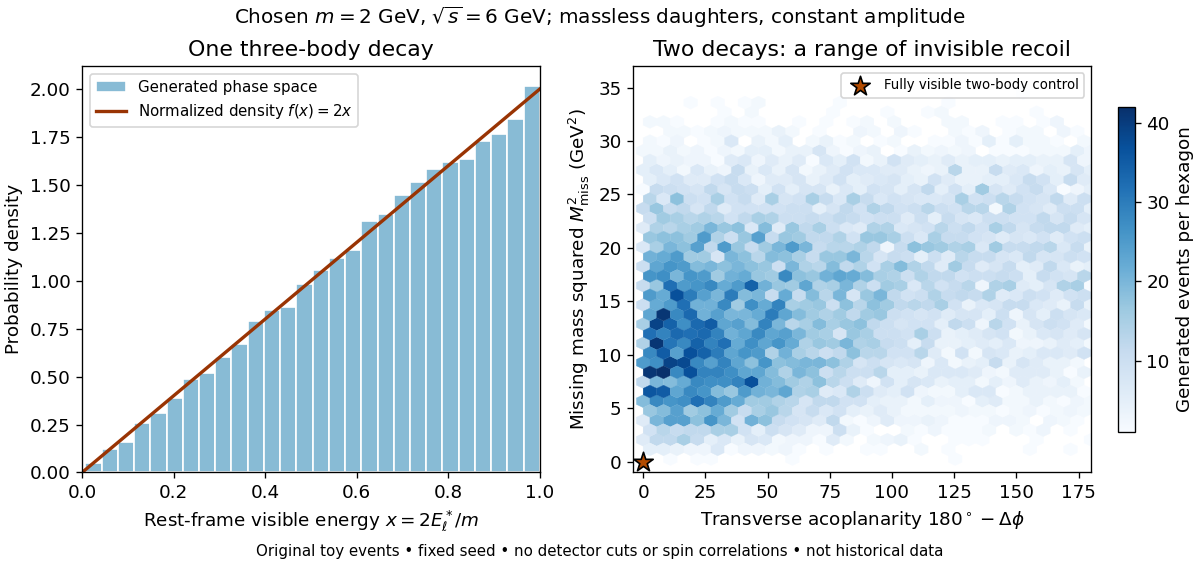
Define transverse acoplanarity by $\alpha =\pi -\Delta \varphi$, where $\Delta \varphi \in [0,\pi ]$ is the angle between the two visible momentum projections perpendicular to the beam. A fully visible two-body event with zero initial transverse momentum has $\alpha =0$ and $M_{\mathrm{miss}}^2=0$. The toy tau lepton events spread away from that point. These observables are complementary: an angular imbalance asks about directions, while the missing invariant mass also uses the visible energies and longitudinal momenta.

A Lorentz-invariant phase space density supplies allowed configurations and their geometric measure. A physical weak interaction decay amplitude reweights them and correlates spins. Consequently the plotted density is a lesson about conservation and available configurations, not a predicted experimental rate or a fit to the discovery sample. The massless charged-daughter approximation is also unsuitable near the muon rest-energy threshold.

For radial mass density $\rho (r)=A{r}^{-2}(1-e^{-r/r_0})$ within radius $R>0$, integration against the spherical volume element gives $M=4\pi ARf(r_0/R)$. The dimensionless quantity $q=r_0/R>0$ hasThus $f$ is positive, strictly decreasing and convex, with $f(0^{+})=1$ and $f(\infty )=0$. Its asymptotic forms are $f(q)=1-q+q{e}^{-1/q}$ near zero and $f(q)=1/(2q)-1/(6q^2)+O(q^{-3})$ at infinity. The density's central $1/r$ divergence is integrable against the factor $r^{2}dr$.

In the usual physics convention for spherical coordinates, the polar angle is the angle between the positive $z$ axis and the position vector. For $r=\sqrt{x^2+y^2+z^2}>0$, it satisfies $\cos \theta =z/r$ with $0\le \theta \le \pi$. The north and south axes have $\theta =0$ and $\theta =\pi$, respectively; the plane $z=0$ has $\theta =\pi /2$. The angle is undefined at the origin. In plane polar coordinates, the same phrase usually denotes the oriented in-plane angle instead, so the reference axis and convention should always be stated. The azimuth supplies the other angular coordinate in three dimensions.

The skin depth is the distance over which a field amplitude falls by $e^{-1}$ inside a conductor. In the local good-conductor limit, $\delta =\sqrt{2/(\mu \sigma \omega )}$. Intensity then falls by $e^{-2}$ over one skin depth; amplitude and intensity penetration lengths differ by a factor two.

For a wave penetrating a nonmagnetic good conductor in the $+z$ direction with time convention $e^{-i\omega t}$, its wavenumber is $k=(1+i)/\delta$, with skin depth $\delta =\sqrt{2/({\mu }_0\sigma \omega )}$. If $\mathbf{E}\parallel \hat{\mathbf{x}}$, Faraday's law of induction gives $\mathbf{H}=[k/({\mu }_0\omega )]E_x\hat{\mathbf{y}}$. Thus the field ratio is $Z_s=E_x/H_y=(1-i)/(\sigma \delta )$, equal to the displayed expression. Magnetic and electric fields have equal exponential penetration lengths but a phasor phase difference $\pi /4$; $H_y$ has the positive phase relative to $E_x$ in this convention.

For an ideal single transit, let the oscillatory magnetic field occupy a region of length $L$, take the longitudinal speed $v$ constant, and neglect edge fields. Each molecule then experiences one square pulse of duration $\tau =L/v$. This is one contiguous interaction region, distinct from the two separated pulses of Ramsey interferometry. The static magnetic field sets the selected transition gap; the transverse drive sets Rabi angular frequency. A change of RF frequency or static magnetic field changes Rabi detuning.

For an original ideal detector model, suppose every successful transition removes an otherwise accepted molecule and the incident beam occupies the lower state of the selected pair. With accepted no-transition signal $S_0$, constant background $S_{\mathrm{bg}}$, and effective loss contrast $0\le \eta \le 1$, writeFor identical trajectories $\overline{P}=P_{g\to e}(L/v)$, giving an intensity dip where transfer is largest. For real trajectory variation, a normalized joint probability density $w(v,ϵ,{\Omega }^{\prime })$ gives the static-offset modelHere $ϵ$ is the trajectory's transition-frequency offset and ${\Omega }^{\prime }$ its drive strength, each in angular-frequency units. The weighting is for molecules accepted by the apparatus, rather than an assumed unfiltered oven distribution. In particular, designing $\Omega L/v_0=\pi$ does not produce a Rabi pi pulse for every speed: at $0.8v_0$ and $1.2v_0$ the resonant transfer probabilities are respectively ${\sin }^2(5\pi /8)\simeq 0.8536$ and ${\sin }^2(5\pi /12)\simeq 0.9330$.

Spread in transit times, static magnetic fields and drive amplitudes can reduce or smear oscillations without quantum decoherence on any individual trajectory. Even the single-transit square pulse has finite spectral width of order $1/\tau$ in angular frequency. If the magnetic field varies substantially along one path, its Hamiltonian operator changes during the passage and the constant-offset average above must be replaced by a time-ordered exponential. Actual molecules may also have several coupled energy levels; the isolated pair and perfect loss discriminator are explicit idealizations of this model.

Insert a complete resolution of identity in energy eigenstates on either side of the time-evolution operator. Each state evolves by its scalar energy phase, yielding the displayed quantum propagator. Its spectral sum includes an integral over any continuous spectrum, with the measure fixed by the continuum normalization. Omitting the scattering states when bound states are also present destroys completeness and the delta-function short-time limit.

A leading principal minor is a principal minor using the first $k$ rows and columns of a square matrix in a specified ordering. Sylvester's criterion uses these minors to characterize positive-definite matrices.

For spin-degenerate Electrons at atomic spacing $a$, alternate the hopping amplitudes $-(t+\delta )$ and $-(t-\delta )$, with $t>0$ and $|\delta |<t$. The doubled primitive unit cell gives an off-diagonal Bloch Hamiltonian entry $-(t+\delta )-(t-\delta )e^{-2ika}$. Its two eigenvalues are the displayed energy bands, for $|k|\le \pi /(2a)$. The band gap at the edge of the Brillouin zone is $4|\delta |$. At half filling there are two Electrons per doubled primitive unit cell, so the lower band is full and the upper empty. This explicit model realizes the period-doubling form of a Peierls distortion.