
For started at a point of radius one, its radial process has the law of the inverse-clock process , where inverts . The logarithmic growth of an exponential Brownian clock with positive drift gives , whereas . Substituting proves the displayed almost sure escape rate and divergence of the radius. Independently, Brownian scaling gives the same rate in probability; if an almost sure logarithmic rate is already known to exist, that identifies its value.
For an -oriented rank- real vector bundle, its Thom class restricts on each fiber to the suspension of the coefficient unit under the oriented identification . Cup product with this class gives the Thom isomorphism. The associated Euler class in a generalized cohomology theory is the pullback along the zero section after forgetting relative supports.
// Target: geometry-and-topology.bigb
Cohomology class of a cooriented submanifold 2026-10-14
An oriented normal bundle of a compact embedded submanifold has a Thom class. A tubular neighborhood and excision identify it with a relative class in . Its image in absolute cohomology is . It restricts to zero off Y and, in an oriented closed ambient manifold, represents the Poincare dual of Y with the normal-first induced orientation.
The logarithmic derivative is periodic under one and decreases by under tau. Integrating around a fundamental cell and applying the argument principle counts exactly one zero, with multiplicity. The displayed zero follows from translating the zero of at . It is consequently simple. For half-integer characteristics only the odd characteristic vanishes at the origin; the other three theta constants are nonzero.
Normal convergence allows termwise differentiation of the defining theta function with characteristics. A tau derivative multiplies a summand by , while its second spatial derivative multiplies it by . This proves the displayed heat equation, linking its lattice-sum construction with diffusion and analytic continuation.
Translation of tau by one gives . Gaussian Poisson summation gives . The square root is the holomorphic branch positive at tau=i. These formulas keep the characteristic phase, which is lost if one states only the transformation of unshifted theta constants.
Jacobi theta duplication identity 2026-10-14
For the binary characteristic convention, each theta function with characteristics has one simple zero per lattice cell. The four zeros of the numerator, at the four half-periods, cancel those of . Their quotient is an entire elliptic function, hence constant. Taking the limit at zero determines the factor one half. The product identity remains valid at the zeros, where the initial quotient requires removable extension.
Period lattice of theta3 over theta4 2026-10-14
Use the radian spatial convention and . Their ratio is unchanged by and changes sign under . The numerator has simple zeros at , while the denominator has simple zeros at . The two sets are disjoint, so any period must lie in , by translating the zero set. The sign rule then gives the displayed exact lattice. Squaring the ratio removes that sign and has precisely the smaller lattice .
Theta constant 2026-10-14
A theta function with characteristics evaluated at spatial argument zero. Its dependence on remains holomorphic. Among the four half-integer characteristic choices, the odd one vanishes identically, whereas the three even constants are nonzero on the half-plane. The zeros of theta functions with characteristics locate their spatial zero away from the origin. Ratios of equal powers of even constants yield the modular lambda function and other modular-invariant functions.
Activity coefficient Created 2026-10-14 Updated 2026-11-05
An activity coefficient expresses departure from a chosen ideal-mixture activity convention. In a concentration-based convention,The thermodynamic activity and coefficient are dimensionless; is the standard concentration. The reference convention fixes which ideal or limiting state has . A mole-fraction convention uses a different ideal activity and must not be mixed silently with the concentration convention.[ref]
IUPAC Compendium of Chemical Terminology, fifth edition (Gold Book) by International Union of Pure and Applied Chemistry. Entries A00115 and A00116, activity and activity coefficient: chemical-potential definition and mixture reference
Substituting activities into an equilibrium constant separates concentration ratios from interaction corrections. For , the correction contains . Changing composition can therefore change an observed concentration quotient even when the thermodynamic constant at fixed temperature and reference state is unchanged. An activity coefficient can be greater or less than one; it is not a fraction of molecules assigned to an active population.
Exponentially large correlation length in a two-dimensional spherical sigma model Created 2026-10-14 Updated 2026-11-05
At and , the weak-coupling renormalization-group flow obeys . Integrating gives . The flow reaches order-one coupling at a length whose logarithm is at this order. Restoring the microscopic scale gives the displayed leading exponential correlation length. Higher loops affect its prefactor, and this conclusion does not apply to the compact model with its Berezinskii–Kosterlitz–Thouless transition.
Thermal cutoff of Lyman-alpha line widths Created 2026-10-14 Updated 2026-11-05
A purely thermal hydrogen absorption line has velocity-space optical depth proportional to with the displayed width. Additional independent Gaussian broadening contributes positive terms to . Fitting the lower envelope of width against neutral-hydrogen column density, with numerical calibration for density and pressure smoothing, estimates the temperature-density relation of photoionized intergalactic gas. A single broad line only bounds the temperature from above when its nonthermal width is unknown.
Thermal diffusion length 2026-10-14
The thermal diffusion length is the characteristic length over which thermal conduction changes a temperature distribution during time in the constant-thermal diffusivity model. It is a scale, not a sharp front or distance travelled at a constant speed: the heat equation has infinite propagation speed mathematically. Different definitions of penetration depth introduce numerical factors. In particular, the normalized one-dimensional heat kernel has spatial variance , so its root-mean-square width is .
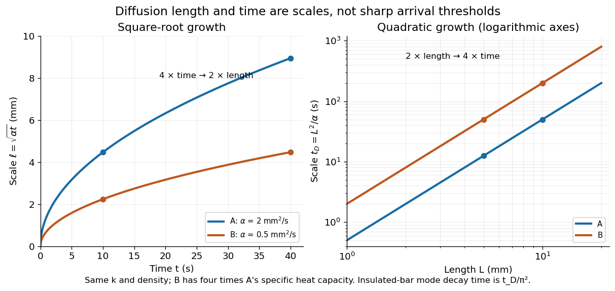
Thermal diffusion length grows as the square root of time; thermal diffusion time grows as length squared
. Original predictions for the two stipulated materials in thermal diffusivity. Left: , with four times the time needed to double length. Right: on logarithmic axes. Equal thermal conductivity with four times the volumetric heat capacity halves the reached length at a given time and quadruples the time at a given length. The scale differs from the insulated-bar decay time by the factor . Details.
At , the model materials have thermal diffusion lengths and . For their thermal diffusion times are and . These values describe the same heat equation as the thermal diffusion rate of a Fourier mode; the different numerical factors come from the definition of the scale.
Thermal conductivity tensor Created 2026-10-14 Updated 2026-11-05
A thermal conductivity tensor relates a temperature gradient to conductive heat flux through . For an anisotropic material, its components can differ between directions, so the heat flux need not be parallel to . Choosing principal axes of a symmetric identifies the principal conductivities.
The local thermal contribution to entropy production isFor passive reciprocal conduction, a symmetric positive-semidefinite gives a nonnegative value; strictly positive conductivities give positive definiteness. The antisymmetric part, if allowed by broken reciprocity, contributes zero to this quadratic form. Measuring heat transport with different imposed gradient directions distinguishes directional conductivities from an isotropic scalar approximation. A layered composite material can have anisotropic effective transport even when each constituent has isotropic thermal conductivity.
If a line bundle on is trivial on each zero-coordinate face, its First Chern class vanishes: the integral second cohomology consists of single-factor second cohomology and cross-products of first cohomology from pairs, and each summand is detected on a coordinate face. The holomorphic exponential sequence then puts the bundle in . The decomposition of first cohomology, including Dolbeault cohomology, identifies this group with . Triviality on the three coordinate axes makes all three factors trivial. Applying this cube principle to the alternating partial-sum pullbacks proves the usual addition-map Theorem of the Cube.
Arithmetic cube identity for Weil heights 2026-10-14
For a line bundle on an elliptic curve over a number field, the geometric cube identity remains exact as a line-bundle identity. The Weil height machine translates it into the displayed bounded-error identity for a chosen logarithmic height, uniformly on the rational triples. This distinction is essential: arbitrary naive heights do not obey an exact quadratic identity. Dividing the identity for by produces an exact identity for the canonical height of an elliptic curve.
Lie derivative of a covariant tensor field 2026-10-14
For a covariant rank-two tensor field, pull back by the flow of a vector field and differentiate at zero flow time. Differentiating the evaluation point produces the first term above; differentiating the two coordinate Jacobians produces the remaining terms. In particular this formula gives the change in a metric tensor under an infinitesimal coordinate displacement. A perturbation defined relative to a fixed background consequently transforms as in the passive displacement convention. The formula applies to symmetric tensors as well as differential forms; tensor symmetry does not make the antisymmetric differential-form formula its definition.
Decomposition of three SU(2) spinors 2026-10-14
For , put , , and . With and inverse , the two-dimensional alternating identity gives . The inverse decomposition is . The symmetric part is the spin- SU(2) representation, and the two independent contractions are spin- representations. This is the spin coupling underlying ground-state three-quark baryons, before the Pauli constraint on three-quark flavour multiplets is imposed.
// Target: quantum-field-theory.bigb
Tensile-crack radiation pattern 2026-10-14
For a planar tensile-crack seismic source, is measured from its normal. The P wave displacement is radial with the first displayed amplitude. The S wave displacement is tangential in the plane containing the observation direction and crack normal, with four alternating signed lobes and nodes at the poles and equator. Both radiative fields depend on the opening rate and vanish once opening stops; the static displacement field depends on the final opening.
Close a three-strand planar tangle and evaluate its reduced Kauffman bracket. The basis has the displayed trace values, with the last value also valid for . Writing braid generators as turns knot-polynomial computations into a five-dimensional algebra calculation.
There are unlisted articles, also show them or only show them.