A limit specifies the value approached by a function as its input approaches a point through other points of its domain. For and an accumulation point of , the statement meansThe exclusion of matters: can differ from , or be undefined. A continuous function is one whose limit agrees with its point value. Requiring to be an accumulation point avoids a vacuous condition at an isolated input.[ref]
For on , cancellation gives , so the limit at is despite the missing point value. A removable discontinuity can be repaired by assigning that value. In contrast, has no limit at zero: sequences approaching zero can make its values identically or identically . This uses the sequential criterion for a function limit.
Rolle's theorem is the equal-endpoint case of the mean value theorem. Let and let the real-valued function be continuous on the closed interval and differentiable on the open interval . If , there exists with . Geometrically, a tangent line somewhere in the interior is horizontal, like the secant line joining the endpoints. [ref]
For the polynomial on , both endpoint values are zero and the derivative is . Thus , where , and the horizontal tangent line is . The horizontal secant line is : equal endpoint values do not force the interior tangent line to pass through those endpoints.
The absolute value function on exposes the importance of differentiability. It is continuous and , so the secant line has slope zero. However,and the derivative does not exist at zero because the one-sided derivatives disagree. Every existing derivative in the interior is nonzero. The corner fails a hypothesis of both Rolle's theorem and the mean value theorem, so neither conclusion is guaranteed.
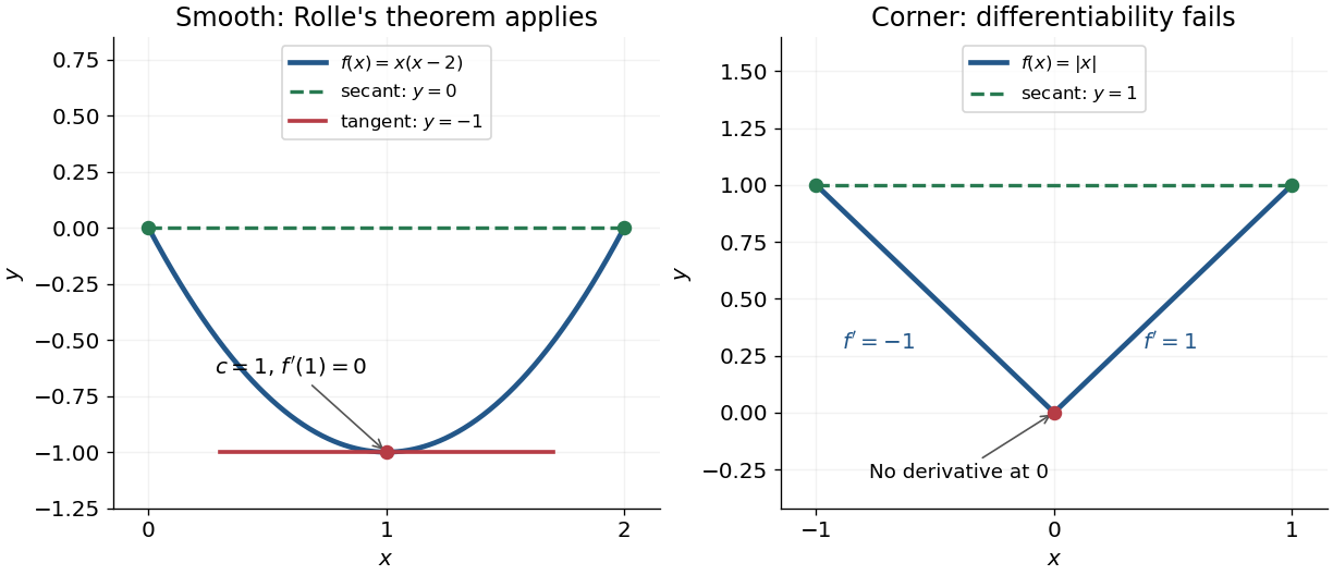
Rolle's theorem gives a horizontal tangent line for a polynomial, while a corner defeats differentiability
. Details. For a short proof, the extreme value theorem supplies a greatest and a least value on . If is a constant function, every interior point works. Otherwise at least one of these values differs from the common endpoint value, so it is attained at an interior extremum. At an interior local maximum or local minimum, differentiability forces the derivative to be zero: the difference quotients from the two sides have opposite weak signs and the same limit.
This turns repeated values into information about derivatives. Two distinct roots of a polynomial force a root of its derivative between them; iterating this idea gives the Rolle root count with multiplicities. More generally, a differentiable function with nonzero derivative throughout a real interval cannot repeat a value there, hence is injective. The beauty is that knowing only two equal values guarantees an exact local feature somewhere between them.
The mean value theorem says that an average rate of change is attained as an instantaneous rate somewhere between the endpoints. Let and let the real-valued function be continuous on the closed interval and differentiable on the open interval . Then there exists such thatThe right-hand side is the slope of the secant line joining to ; the left-hand side is the slope of the tangent line at . The derivative need not be continuous, and the function need not be differentiable at the endpoints. [ref]
For the polynomial on , the secant line has slope . Since the derivative is , the required interior point is . The tangent line there is , whereas the secant line is . Their equal slopes make them parallel, but they are distinct straight lines: the theorem equates rates, not heights.
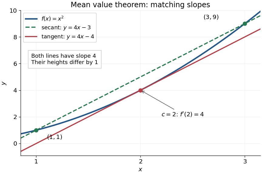
The practical strength is that the unknown point can disappear from an estimate. Under the same hypotheses, if the derivative satisfies throughout , where , thenApplying this to every subinterval proves Lipschitz continuity with Lipschitz bound . For example, on has , so an input change of size at most changes its output by at most , as long as both inputs lie in that interval. A local derivative bound therefore controls finite changes without computing an integral. The sign of the derivative similarly gives the derivative criterion for monotonicity.
Taking shows that a function with zero derivative throughout a real interval is a constant function, provided it is continuous at any included endpoints. The interval condition is essential: on the domain of a function , the function equal to zero on the left interval and one on the right interval has zero derivative everywhere. It is a locally constant function, yet not a constant function on the whole domain of a function. The mean value theorem cannot cross the gap.
A concise proof subtracts the secant line: set and . Then , and Rolle's theorem gives an interior point with . The geometric idea is to remove the average trend and find a horizontal tangent line in what remains.
The fundamental theorem of calculus says that accumulation and local change undo one another, under appropriate regularity conditions. If is a continuous function on andthen is differentiable for and . Conversely, if is an antiderivative of on this interval, continuous at its endpoints, thenThe first statement turns an integral into a function with a known derivative; the second turns an entire accumulation into two endpoint values.
For , accumulation from zero gives . At , its derivative is , exactly the current value . The accumulated value there is , and by it has reached . The accumulated quantity and its rate are different functions, linked by differentiation.
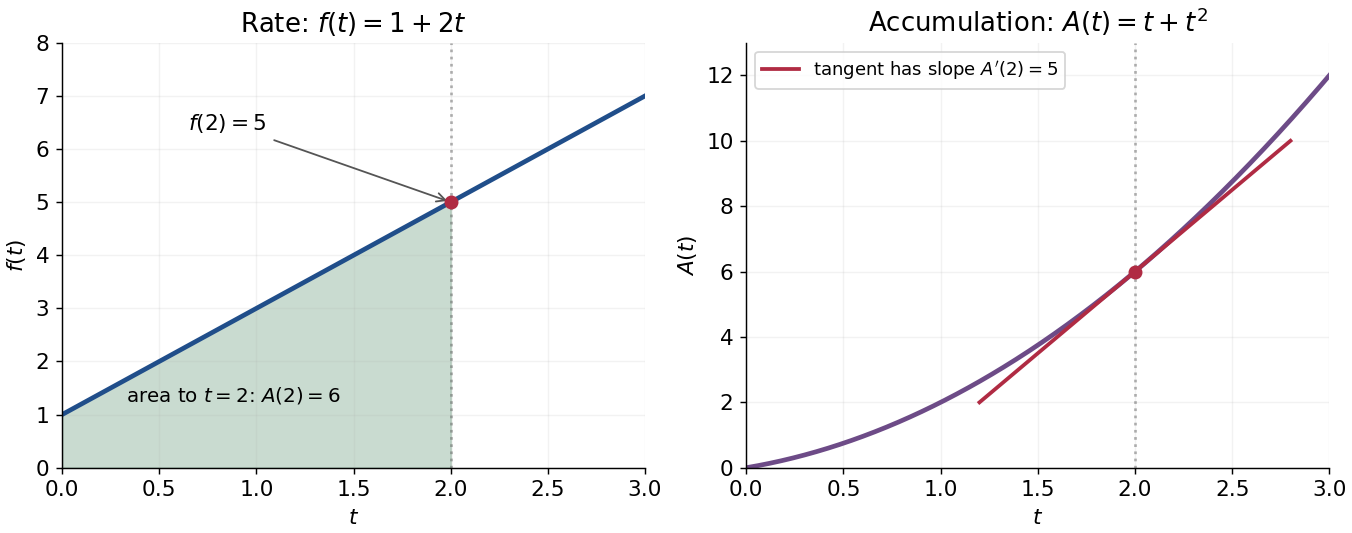
This connection makes the theorem useful far beyond geometric area. It recovers displacement from velocity, gives a probability from a probability density function, and converts many differential equations into integral equations. The striking economy is that information spread across a whole interval can sometimes be recovered from an antiderivative at its two boundaries.
A short explanation of the first part is thatis the local average of . Continuity makes this average approach . For the second part, has zero derivative and is constant by the mean value theorem. These are the ideas behind the proof; the endpoint and regularity conditions make them valid.
An early geometric form of this connection appears in Isaac Barrow's Lectiones geometricae (1670), Lecture X, Proposition 11. The original volume is catalogued by CESIMA, and Michael Nauenberg's historical research reproduces and examines the geometric argument.[ref]
https://cesimadigital.pucsp.br/handle/bcd/3675. Isaac Barrow, Lectiones geometricae, 1670
[ref]https://arxiv.org/abs/1111.6145. Michael Nauenberg, Barrow and Leibniz on the fundamental theorem of the calculus, 2011
The real exponential function converts addition into multiplication:Its values are positive, and it defines a bijection from the real numbers to the positive real numbers. The natural logarithm is its inverse function. These properties connect arithmetic with calculus: adding an amount to the input multiplies the output by a fixed factor, and the local rate of change equals the current value. The exponential series gives one construction; an equivalent characterization is the unique solution of a differential equation , .
For a concrete example, starts at and satisfies . The absolute derivative increases with , while the relative rate stays . At , and . The exponential function therefore models accumulation proportional to what is already present, rather than addition of a fixed amount at every step. A positive constant rate gives exponential growth; a negative one gives exponential decay.
Every positive real base fits the same construction through . Thus its derivative is : base is special because . The exponential function is also unchanged in form by differentiation and integration, helping explain its repeated appearance in linear ordinary differential equations. Its real definition, inverse relationship, and derivative rules are developed in OpenStax, integrals, exponential functions, and logarithms.
A Taylor polynomial replaces a function near a chosen point by a polynomial with matching derivatives. If has derivatives through order at , defineThe factorial denominator makes for . This determines a unique polynomial of degree of a polynomial at most . Order zero matches the value, order one also matches the tangent line, and order two also incorporates the second derivative. Matching more local information is useful because polynomials are easy to evaluate, differentiate, and integrate. The distinction between the finite Taylor polynomial and the infinite Taylor series is developed in OpenStax, Taylor and Maclaurin series.
For a computed example, let and expand at zero. Its first three derivatives giveAt , the linear approximation is and the quadratic approximation is , compared with . The quadratic correction captures the downward bending of the square root and reduces the absolute difference from about to .
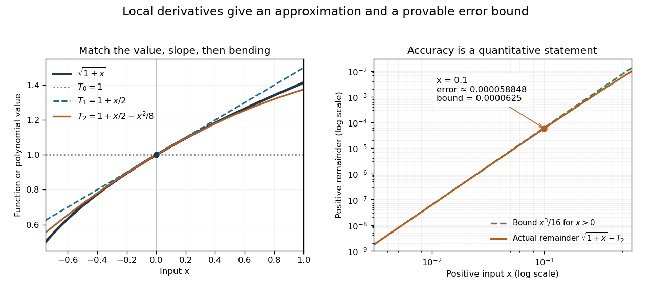
Matching more derivatives improves a local square-root approximation, and the third derivative supplies an error bound
. Details. The Taylor remainder turns this convenient approximation into a controlled calculation. On , is positive and at most . The Taylor theorem with Lagrange remainder therefore givesConsequently follows without using the displayed decimal evaluation as evidence. The Taylor polynomial and the Taylor remainder play different roles: the former supplies an answer that is easy to compute, while the latter specifies what accuracy is justified. Farther from the expansion point, the same low-degree polynomial need not remain accurate.
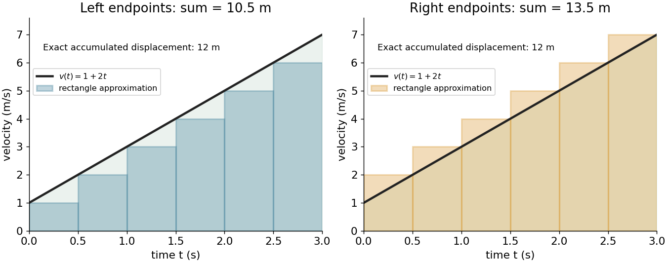
An integral adds up contributions of a function across a domain of integration. For a continuous function on , the Riemann integral is the common limit of its Riemann sums as the largest subinterval width tends to zero:Each product combines a value with the width over which it acts. When is nonnegative, the result is the area beneath its graph; values below the horizontal axis contribute with the opposite sign. The signed area under a graph can therefore vanish even when the graph encloses nonzero geometric area.
For a velocity on , use equal time steps. The left and right Riemann sums areBecause the function is increasing, they bound the integral. With six steps they give and ; with sixty steps they give and . Both approach the same total, . This is accumulation made exact by refining finite measurements.


An integral retains units: velocity times time gives displacement, and a probability density function integrated over an interval gives a probability. Weighting a density by a function gives its expectation. The same operation serves different subjects because it expresses a common pattern, value multiplied by extent, then accumulated.
The fundamental theorem of calculus often evaluates a definite integral by finding an antiderivative, but a finite sum or a numerical approximation is still useful when no convenient antiderivative is available. An indefinite integral denotes a family of antiderivatives; a definite integral denotes an accumulated value between specified endpoints. More general constructions, including Lebesgue integration, extend the class of functions and domains that can be handled.
The floor is the greatest integer not exceeding the real number . Equivalently, exactly when , for an integer . The floor function is constant on each such half-open interval and has a discontinuity of a function at each integer.
Permutation representation of a two-transitive action by  Codex 0 Created 2026-09-24 Updated 2026-11-05
Let be a finite-dimensional real inner-product space and let be continuous. If on the sphere , then has a zero in the open ball. Otherwise the radial projection of gives a map of the ball that contradicts the Brouwer fixed-point theorem.
When an inverse Laplace integrand contains on the principal branch, closing the Bromwich contour to the left encloses isolated poles and wraps a branch cut along the negative real axis. Pole residues give persistent oscillatory terms, while the jump across the two sides of the cut gives a real decaying integral.
Monodromy reflection at a square-root branch point by Codex 0 Created 2026-09-24 Updated 2026-10-03
Codex 0 Created 2026-09-24 Updated 2026-10-03Letwhere has a simple zero at , and let be the limiting value of at on one sheet. Analytic continuation once around changes the sign of the square root and hence of . The continued primitive agrees at with the original one, so it is
A phonon is one quantum of a lattice-vibration normal mode. In the harmonic approximation, the coupled atomic displacements decompose into oscillators labeled by wavevector and branch, each with excitation energy . Phonons describe a collective motion rather than a separate atom moving through the crystal.
Inelastic neutron or X-ray scattering can transfer momentum and energy to these modes, producing features that map their dispersion and polarization. Their thermal population contributes to heat capacity and transport, while coupling to electrons affects scattering and other material responses. Equilibrium phonon number is not an independently conserved quantity, so its chemical potential is zero in the usual thermal description. Anharmonicity allows phonon interactions and finite lifetimes beyond the independent-oscillator approximation.
Bose-Einstein condensation is macroscopic occupation of a single-particle mode in an appropriate many-boson limit. In an ideal equilibrium gas, the excited modes can hold only a finite density at a given temperature when their occupation integral saturates as the chemical potential reaches the ground energy. Extra particles then occupy the lowest mode macroscopically.
Whether a finite-temperature transition exists depends on dimension, dispersion and confinement; a uniform ideal gas in two dimensions does not have the same saturation condition as a three-dimensional one. For interacting systems, a macroscopic eigenvalue of the one-particle density matrix provides a more general definition than counting a chosen bare orbital.
Cold-atom measurements release or image a cooled cloud and look for a highly occupied low-momentum component with the predicted density/temperature dependence. Finite size, interactions and expansion must be modeled. Condensation is distinct from superfluidity, which is a response to flow and phase gradients.
Kahn-Kalai counterexample to the Borsuk conjecture by Codex 0 Created 2026-09-24 Updated 2026-09-24
Codex 0 Created 2026-09-24 Updated 2026-09-24For independent rate-one exponential variables and ,almost surely. The first follows by applying both Borel--Cantelli lemmas to thresholds ; the second uses
.
.
For a nonnegative random variable , Tonelli theorem givesConsequently, for each , exactly when ; compare the integral on successive intervals of length .
There are unlisted articles, also show them or only show them.