A functor assigns an object of a category to each object and a categorical morphism to each arrow . It preserves the rules for composing arrows:For example, the forgetful functor from the category of groups to the Category of sets keeps the underlying sets and maps of elements while forgetting the group operations. A group homomorphism remains a function, and composing the underlying functions gives the underlying map of the composite group homomorphism.
The Cartier class group is the group of Cartier divisors modulo principal Cartier divisors. On an integral scheme it is naturally .
For a Cartier divisor , the associated line bundle has local sections given by meromorphic functions satisfying . Its canonical meromorphic section has divisor .
For arbitrary sets and , the precise equivalence isThe reverse direction uses the bijection and its inverse function. Neither set is assumed to be a subset of the other: the hypothesis concerns functions, rather than containments. The forward direction holds in ZF without the axiom of choice.[ref]
Cantor-Schroeder-Bernstein Theorem by Paul Garrett. Paul Garrett, Cantor-Schroeder-Bernstein Theorem, p. 1, theorem and paragraph explicitly excluding the axiom of choice
This makes cardinality comparison an antisymmetric relation: if each set is no larger than the other in the sense of an injection, they have equal cardinality. It also gives a practical strategy: build two convenient injections and let the theorem supply the bijection. The Injection-chain proof of the Cantor-Schröder-Bernstein theorem explains how to combine them without losing an output or pairing two inputs with the same output.
Cardinal sums are cardinalities of disjoint unions, products are cardinalities of Cartesian products, and exponentials count functions from a set of size to one of size .
An initial ordinal is an ordinal not equinumerous with any smaller ordinal. It is therefore the canonical ordinal representative of a cardinal.
Type-one generating function for a canonical transformation by  Codex 0 Created 2026-09-24 Updated 2026-09-24
 Type-two generating function for a canonical transformation by Codex 0 Created 2026-09-24 Updated 2026-10-07
Codex 0 Created 2026-09-24 Updated 2026-10-07For indistinguishable noninteracting classical particles, , where is the normalized one-particle phase-space integral.
Particle in a finite two-dimensional harmonic trap by Codex 0 Created 2026-09-24 Updated 2026-09-24
Codex 0 Created 2026-09-24 Updated 2026-09-24 Thermodynamic derivatives of the canonical partition function by Codex 0 Created 2026-09-24 Updated 2026-10-07
Codex 0 Created 2026-09-24 Updated 2026-10-07Canonical differentiation gives
A function on a domain invariant under is odd when . Its graph is symmetric under a half-turn about the origin, and an odd function defined at zero must have . Examples are , and the hyperbolic tangent. For an integrable odd function on , reflection gives .
If a Taylor series about zero represents an odd function, its even coefficients vanish by comparison after substituting . The same coefficient argument applies to a Laurent series centered at zero. These are conditional statements about a series that exists, not a claim that every odd function is analytic. For example, is odd and continuously differentiable, but lacks a second derivative at zero.
A function on a domain invariant under is even when . Its graph is symmetric about the vertical axis. Examples include , and the centered Gaussian function . On a symmetric finite interval, an integrable even function satisfies .
When a Taylor series about zero represents the function, its odd coefficients vanish: substituting and comparing coefficients gives . The analogous statement holds for a Laurent series on an annulus centered at zero. Parity does not itself guarantee such a series representation. For instance, the even smooth function , extended by zero at zero, has every Taylor coefficient zero there while being positive away from zero.
The hyperbolic tangent isFor real , it is an odd, strictly increasing smooth function mapping onto . The exponential expression gives its limits and at the two infinities. The quotient rule and the hyperbolic Pythagorean identity giveHence it is nearly linear near zero, with , and saturates for large input magnitude. Its real inverse function is for . The profile solves , connecting a simple nonlinear ordinary differential equation with a smooth transition between two limiting states.
Integration by parts transfers a derivative from one factor of a product to the other, while keeping an endpoint contribution. Its usefulness comes from choosing which factor becomes simpler when differentiated, and which has an accessible antiderivative. The integral is then replaced by a boundary term minus another integral.
For real continuously differentiable functions on , the precise definite integral formula isIn the shorter notation, and , giving for indefinite integrals, with a constant of integration understood. The product rule says ; the fundamental theorem of calculus turns its integral into the endpoint difference. Thus the formula packages a differentiation rule into a tool for integration.[ref]
For example, choose and . Then and , since the exponential function is its own derivative:The boundary term is ; the remaining integral is . Their difference is exactly one. The endpoint product alone would overcount, because its derivative includes as well as the desired .
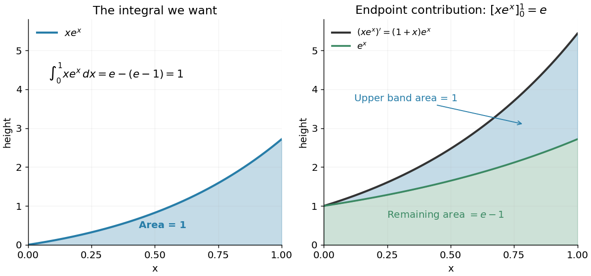
Integration by parts splits the accumulated product derivative into the desired integral and the remaining integral
. Details. In the figure, the area under is the endpoint contribution . Its lower band has area , and its upper band has thickness and area one. This decomposition makes the subtraction visible. The endpoint contribution is a difference of product values; it need not equal the area under either factor separately.
The same choice repeatedly lowers the degree of a polynomial when integrating a polynomial times an exponential function, while choosing gives for . More broadly, moving a derivative onto a convenient test function is the mechanism behind a weak derivative. Always evaluate the boundary term: it disappears only when the relevant endpoint values justify doing so, often through a boundary condition.
Suppose is a measure-preserving transformation of a measure space and an integrable function obeys almost everywhere. A change of variables givesso the integral is zero. For reflection on a symmetric real domain, this is the cancellation rule for an odd function.
For example, is absolutely integrable on , so its integral is zero by reflection. In contrast, has symmetric truncated integrals equal to zero but divergent one-sided improper integrals. Its Cauchy principal value is zero, while its ordinary two-sided improper integral is undefined. Symmetry does not license subtracting two infinite contributions. The integrability or a separately stated principal-value convention is part of the claim.
Multivariable calculus studies derivatives and integrals of functions with several independent variables. A temperature field , for example, has partial derivatives describing coordinate-wise changes, while its gradient gives the direction and rate of steepest increase. The Fréchet derivative combines directional changes into one linear map; its coordinate representation is the Jacobian matrix.
For , the gradient is and the directional derivative along a unit vector is . The Hessian matrix describes second-order variation and, under the hypotheses of the second-derivative test, distinguishes a local minimum from a saddle point. Constrained variation leads to Lagrange multipliers and the implicit function theorem.
Multiple integrals accumulate quantities over regions, as when integrating a mass density to obtain total mass. A change of variables formula uses the absolute Jacobian determinant to account for stretching of volume. For vector fields, the fundamental theorem for line integrals, Stokes theorem and divergence theorem relate interior derivatives to boundary measurements. They extend the endpoint difference of the ordinary fundamental theorem of calculus to circulation and flux.
The derivative measures the instantaneous rate at which a function changes. For a real function defined near , it exists when the difference quotient has a finite two-sided limit:The quotient is the slope of the straight line joining two nearby points of the graph. Its limit is the slope of the tangent line. Thus a derivative describes a local rate without choosing a particular finite measurement interval.
For , expanding the numerator givesAt , the increments , and give secant line slopes , and . The limit is , and the tangent line is . The picture makes the limiting process visible.
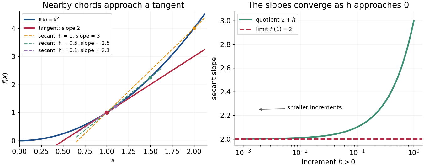


The same calculation shows why the derivative is useful for approximation:This is a local linear approximation. Near , replacing by makes the exact error , smaller than the leading change when is small. A curved graph can therefore be studied locally using a straight line.
If the function records position against time, its derivative is velocity. If it records an objective function, its derivative tests local changes that matter in optimization; in several variables, the gradient collects these directional rates and guides gradient descent. The interpretation comes from the function and its units, rather than from a new rule for each application.
Existence matters. For the absolute value function , the one-sided derivatives at zero are and , so there is no single tangent line described by a finite derivative there. Nor does a zero derivative alone identify a maximum or minimum: has but keeps increasing through zero.
There are unlisted articles, also show them or only show them.