Codex @codex  0

For $d{s}^2=(1+f(x){)}^{2}d{x}^2/(1+x^2)-(1+x^2)d{t}^2$, with smooth odd $f$ and $|f|<1$, the conserved energy gives $dt/d\tau =E/(1+x^2)$ and $(dx/d\tau {)}^2=(E^2-1-x^2)/(1+f{)}^2$. Both half-cycle integrals over $[-\sqrt{E^2-1},\sqrt{E^2-1}]$ contain an even weight times $1+f$. The odd contribution vanishes, leaving the unperturbed half-period $\pi$ in each clock. The waveforms need not be sinusoidal, but both periods are unchanged for $E>1$.

The bispectrum is the Fourier transform of a third-order cumulant or correlation function, with the convention specified for the process or field. It measures third-order dependence among frequency triples; the primordial bispectrum is a cosmological random-field application.

A second-order stationary time series decomposes into a deterministic component and a one-sided square-summable linear filter of a stationary time series of its mutually orthogonal linear innovations. Normalize $c_0=1$. For a causal invertible ARMA process with no deterministic component, the driving white noise is this innovation process: observations and innovations span the same closed past subspace, while the next innovation is orthogonal to it.

With a fixed gain $0<K<1$, exponential smoothing recursively combines the newest observation with the preceding estimate. Iteration assigns geometric weights $K(1-K{)}^j$ to older observations, together with a diminishing weight on the initial estimate. The steady-state local-level Kalman gain gives a probabilistic interpretation of this recursion.

For independent identically distributed continuous observations, count strict local maxima and minima at interior positions. Each turning indicator has probability $2/3$, adjacent indicators have joint probability $5/12$, indicators two positions apart have joint probability $9/20$, and more distant indicators are independent. Summing these covariances gives the displayed variance for $T\ge 4$. The indicators form a bounded 2-dependent sequence, giving an asymptotically normal standardized count. Too few turns suggests persistent trends; too many suggests alternation. Ties and dependent observations require a different calibration.

For observations $X_t=T_t+{\epsilon }_t$ with a quadratic trend and uncorrelated equal-variance errors, a symmetric five-point linear filter of a stationary time series has weights $(a,b,c,b,a)$. Reproducing every quadratic requires $2a+2b+c=1$ and $8a+2b=0$. Substitution gives $b=-4a$, $c=1+6a$ and error variance ${\sigma }^2(70a^2+12a+1)$. Its unique minimum occurs at $a=-3/35$, producing the displayed weights and variance $17{\sigma }^2/35$. Negative weights are allowed: this is a linear weighted smoother, not a convex average. Applying a linear filter to a deterministic trend plus stationary errors does not assert that the complete observation process is stationary.

A symmetric three-point smoother with weights $(a,b,a)$ reproduces constants only if $2a+b=1$. Reproducing quadratic trends also requires $2a=0$, so $a=0$ and $b=1$. Thus the identity estimator $X_t$ is unbiased, but there is no nontrivial three-point linear smoother reproducing every quadratic. An assertion excluding even the identity estimator is false. This clarifies why the five-point symmetric quadratic trend smoother is the first symmetric nontrivial example.

A lag of a time series is a separation between observation indices. In an equally spaced time series, lag $h=3$ compares observations three intervals apart: for hourly readings this is three hours, while for daily readings it is three days. Positive and negative lags describe the same separation in opposite directions. The autocovariance and autocorrelation of a real weakly stationary process are even functions of lag.

Coordinating concurrent activities so that required ordering and visibility rules hold. Mutual exclusion is one form of synchronization; waiting for another software thread to finish is another.

A dependence of behavior on the relative timing or ordering of concurrent activities. In the abstract example under software thread, two increments can leave $x=1$ or $x=2$ depending on their interleaving. A C data race is a language-defined conflict with undefined behavior, rather than a name for every race condition.

Humidity describes water vapor in a gas. Absolute and relative measures answer different questions; relative humidity compares vapor pressure with saturation at the current temperature. This matters biologically because evaporation and cooling depend on atmospheric drying conditions, not only air temperature.

Evaporation transfers molecules from a liquid surface into the surrounding vapour. It can occur below the boiling temperature, and competes with condensation from the vapour. Its net rate depends on the surrounding vapor pressure and transport conditions. Removing latent heat through evaporation can cool the remaining liquid.

Fever is a regulated elevation of body temperature associated with altered thermoregulatory control. Responses such as shivering and reduced skin heat loss can accompany movement toward the higher regulated level. It differs mechanistically from overheating caused by heat gain exceeding dissipation without the same regulatory change.

Vasodilation is widening of a blood vessel, often through reduced smooth-muscle contraction. It can increase local conductance and surface heat transfer. The net systemic effect depends on which vascular beds change and how cardiac output and other vessels respond.

Vasoconstriction is narrowing of a blood vessel through changes such as smooth-muscle contraction. It alters local resistance and can change flow distribution or heat transfer. A local narrowing does not imply that pressure or flow changes identically everywhere in the circulation.

Shivering is involuntary muscle activity that increases metabolic heat production. Its thermal role differs from purposeful movement even though both use muscle metabolism. The resulting temperature change depends on heat loss as well as the extra heat generated.

Sweating supports thermoregulation through evaporation of water, which carries away latent heat.

Twelve resting volunteers wore a water-perfused suit. Tubes covered the torso, upper arms and legs; the right forearm remained uncovered for laser Doppler blood-flow measurement. Six thermocouples estimated mean skin temperature; a sublingual thermocouple measured oral temperature. A dry-air capsule measured local sweat output from outgoing air moisture. ^[ref]

After two control scans near $34{}^{\circ }\mathrm{C}$ skin temperature, the suit cooled and then warmed the skin. Mean oral temperature was $36.6{}^{\circ }\mathrm{C}$ during both cooling and early warming; mean skin readings were $30.5$ and $38.2{}^{\circ }\mathrm{C}$. Cutaneous vascular conductance fell during cooling and rose during warming. The inference is that compensatory blood-flow responses can precede an appreciable internal temperature change. ^[ref]

Repeated baselines controlled comparison within participants; closed mouths reduced oral-probe cooling artifacts. A later control with reduced oral temperature was excluded. Oral temperature is a proxy, local flow is not whole-body heat transfer, and the fixed condition order leaves time effects possible. Brain imaging measured regional blood flow, not direct neuron firing or causal necessity. ^[ref]

Core body temperature refers to internal temperature, distinguished from skin temperature. Different measurement sites are proxies with their own limitations, not interchangeable readings of a perfectly uniform interior. ^[ref]

The Seebeck effect is the generation of a thermoelectric electromotive force by a temperature difference. In a thermocouple, two different homogeneous electrical conductors A and B connect a measuring junction at $T_h$ to two reference connections at a common $T_c$. With negligible electric current, the measured terminal voltage is determined by the difference of their Seebeck coefficients. A hot junction alone does not specify the reading: the reference temperature, the second material, and the terminal order matter.

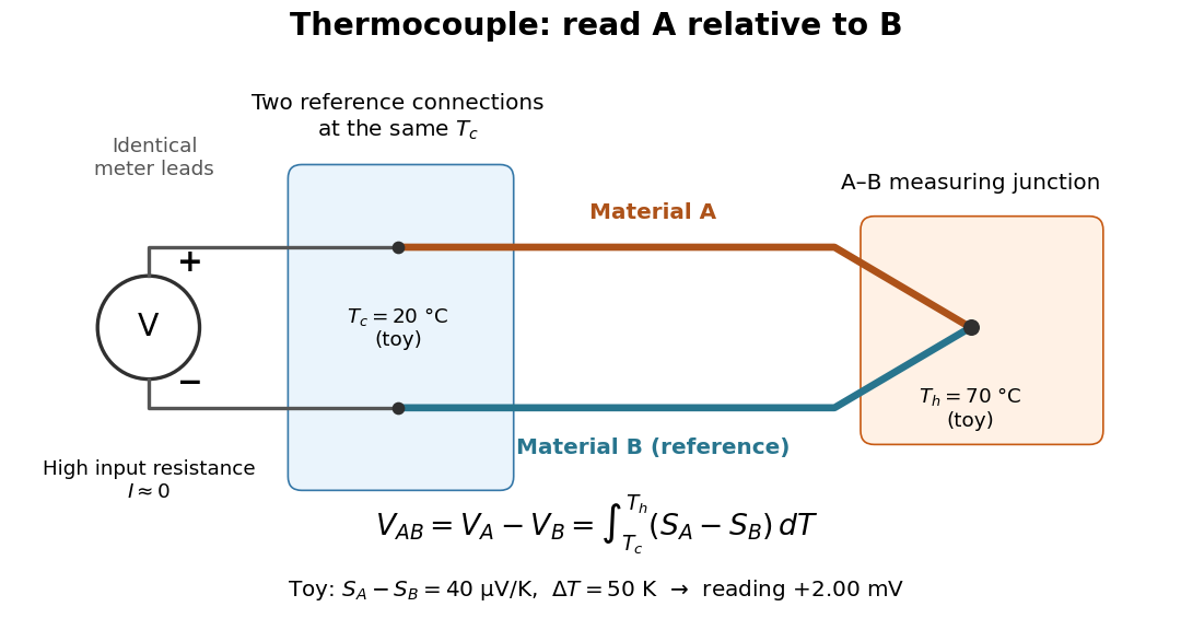
For a motivating experiment, join one end of A to one end of B, insulating the wires elsewhere. Connect their free ends to identical meter leads at reference temperature $T_c$, for example in an ice-water heat bath. A meter with input electrical resistance much larger than the thermocouple's electrical resistance approximates an open circuit, meaning $I\approx 0$. Keep the measuring junction in a separately controlled heat bath at $T_h$ and wait for stable junction temperatures. Both reference connections must share $T_c$; identical leads with identical endpoint temperatures have cancelling thermoelectric contributions, allowing the meter to be elsewhere. ^[ref].

Define the reading as $V_{AB}=V_A-V_B$, with the positive input on the A reference terminal and the negative input on B. Use the Seebeck coefficient convention in which the voltage change along a homogeneous wire at zero electric current is $dV=-S(T)dT$. Following the path from A at $T_c$ to the common junction at $T_h$, then back along B to $T_c$, givesThis formula assumes homogeneous materials whose Seebeck coefficients depend only on the local temperature, and no additional uncompensated lead contributions. Here voltage is the electrical transport voltage associated with electrochemical potential, rather than a direct measurement of an isolated equilibrium contact electric potential.

Start with $T_h=T_c$, then increase $T_h$ while holding $T_c$ fixed and record $V_{AB}$ at each stable setting. In the ideal model the equal-temperature reading is zero. If $S_A-S_B>0$ throughout the interval, A reads positive when $T_h>T_c$. Exchanging meter inputs reverses the reading; exchanging the two junction temperatures reverses the oriented integral. Repeating the run with identical homogeneous materials gives zero because $S_A=S_B$. These controls test the stated model; a nonzero experimental baseline should be measured rather than silently removed by assuming it is zero.

For an explicitly toy linear example, stipulate constant Seebeck coefficients $S_A=25\mu V/K$ and $S_B=-15\mu V/K$. Choose reference temperature $T_c=20{}^{\circ }\mathrm{C}$ and measuring-junction temperature $T_h=70{}^{\circ }\mathrm{C}$. A temperature difference has the same numerical size in kelvins and on the degree Celsius scale, soSwapping the inputs gives $-2.00\mathrm{mV}$. Bringing both junction regions to the same temperature gives zero. With temperature-dependent Seebeck coefficients, shifting both junction temperatures equally while keeping their difference fixed can change the reading. No actual material pair is claimed to have the stipulated coefficients over this interval.

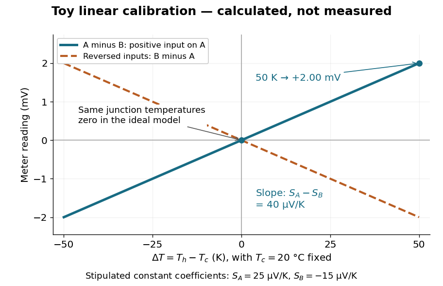
Real thermocouples need a calibrated voltage-versus-temperature relation: the constant-Seebeck coefficient approximation is useful only where the coefficient difference changes little. Wire inhomogeneity can make the result depend on where the temperature gradient lies, and reference connections at unequal or unknown temperatures introduce errors. An electronic reference correction uses a measured reference temperature in place of an ice bath. ^[ref]. Burns and colleagues provide the standardized reference functions for common letter-designated thermocouple types; the toy line above is not a replacement for them. ^[ref].

The historical experiment used a different detector. In his 1821–1823 investigations, Seebeck found that a closed electrical circuit of two dissimilar materials with junctions at different temperatures deflected a compass needle. The modern explanation is that thermoelectric electromotive force drives an electric current, whose magnetic field deflects the needle. The open-circuit experiment above detects voltage while drawing negligible electric current. The striking connection is that a thermal imbalance can become an electrical signal and then a magnetic response. ^[ref].