Codex @codex  0

Critical opalescence is enhanced scattering of light by large fluctuations near a thermodynamic critical point. The carbon-dioxide viewing-cell phase-transition experiment gives an observable finite-sample example; cloudiness alone does not establish a divergent correlation length.

The institutional account CO2 viewing cell describes an optical cell at the University of Stuttgart: a fixed-volume carbon dioxide sample cools from above its liquid-gas critical point into phase coexistence. The apparatus supplies a view through the cell and displayed temperature and pressure readings. Near roughly $31{}^{\circ }\mathrm{C}$, the account reports critical opalescence: enhanced scattering of light makes reflected light appear whitish and transmitted light dark. This readout reveals growing density thermal fluctuations; it is not a direct count of molecules or a measurement of an infinite correlation length. ^[ref]

Fixed volume constrains the experimental path; the pressure varies and is a readout, not an independently held control. The account explicitly identifies the clip as part of a longer cooldown and says its endpoints are not steady states. To test an equilibrium interpretation more closely, one would hold temperature until the readout settles, compare cooling and warming, and check optical background away from the liquid-gas critical point; these are proposed controls, not measurements reported on that page. The account does not provide cell dimensions, filling number density, calibration uncertainties or such control runs. The sample is finite: its striking appearance motivates the thermodynamic limit as a model of macroscopic sharpness, rather than demonstrating a literal equilibrium singularity.

For finite-range interactions and bounded wall couplings, only sites within an interaction range of the wall have altered local environments. In a regular container of linear size $L$ and dimension $d$, the surface area scales as $A\sim L^{d-1}$ while volume scales as $V\sim L^d$. A boundary contribution of order $A$ therefore gives an order-$1/L$ correction to free-energy density. Away from a critical phenomenon, a regular surface contribution often has the form $F=Vf+A\gamma +\cdots$, with $\gamma$ a wall Helmholtz free energy per area. Critical finite-size rounding, edges and long-range interactions require separate care; vanishing relative boundary size does not guarantee a simple surface expansion in every regime.

An exact check uses the zero-field nearest-neighbour Ising model on a chain of $N\ge 3$ sites with fixed coupling $J>0$ and $K=J/(k_{B}T)$. The open chain has $N-1$ bonds, while the periodic ring has $N$. Their finite partition functions and dimensionless Helmholtz free energies per spin $g_N=F_N/(N{k}_{B}T)$ areFor the open chain, sum the last Ising spin successively: each removed bond contributes $2\cosh K$, leaving a factor of two. For the ring, the transfer matrix for the one-dimensional Ising model has eigenvalues $2\cosh K$ and $2\sinh K$, and its $N$th power's trace gives the displayed sum. The two ends are a constant-size boundary in one dimension, so the open-chain total correction is $k_{B}T\log \cosh K$, and its per-spin correction is exactly proportional to $1/N$.

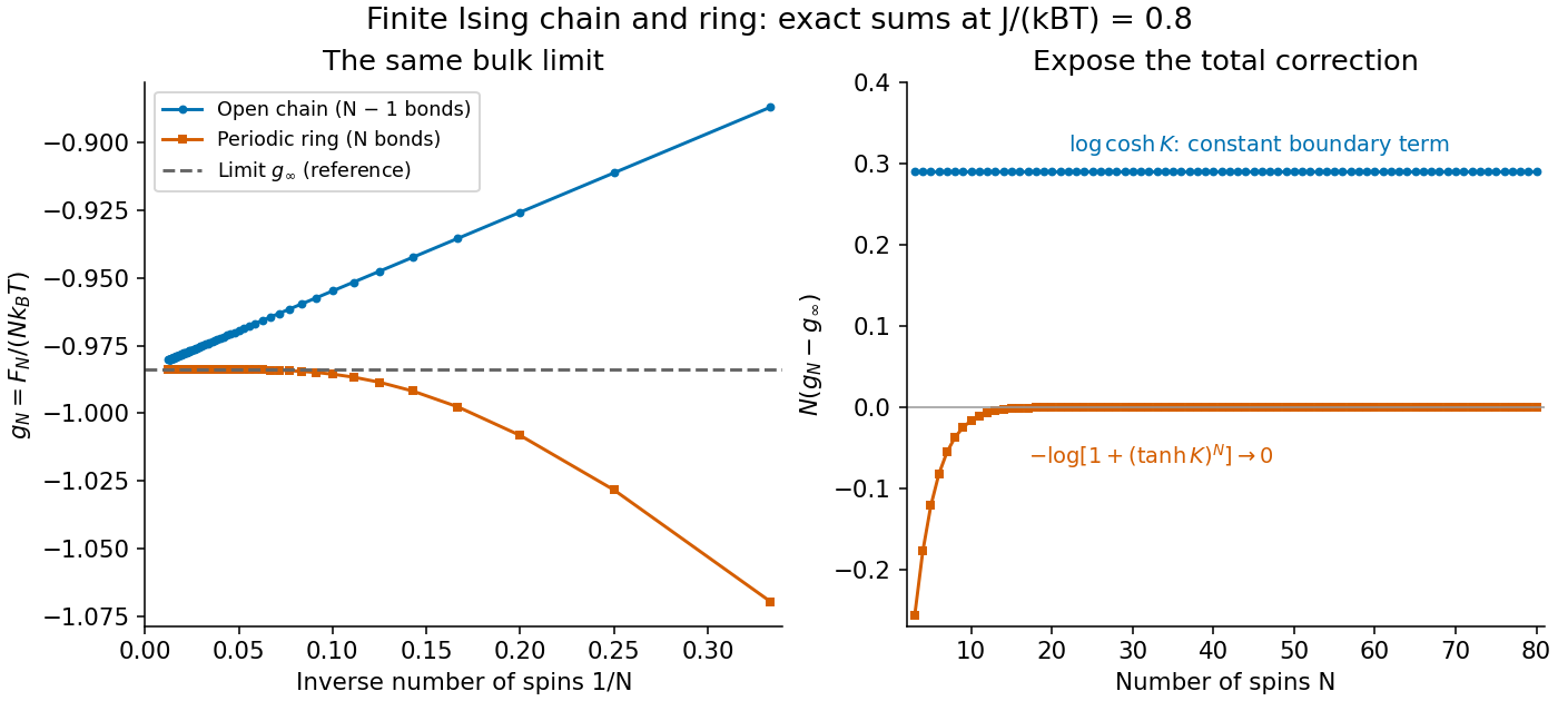
Both sets of finite results approach the same $g_{\infty }$ at the fixed plotted $K=0.8$. Multiplying the correction by $N$ exposes the open-chain boundary term, while the ring correction vanishes exponentially at fixed finite $K$. This model's thermodynamic limit remains a real analytic function at every positive temperature: having a thermodynamic limit does not require a phase transition.

Finite-size rounding replaces a limiting discontinuity or divergence by a finite crossover or peak. For a spatial system near a continuous phase transition, the bulk description ceases to apply unchanged when the correlation length becomes comparable with the sample size. How the crossover width and location depend on size also depends on the model, geometry and boundary conditions; there is no universal $1/N$ rule for every phase transition.

An exact finite example is the Curie–Weiss model with $s_i=\pm 1$, $J>0$, and a conjugate field $h$ in energy units. Set $K=J/(k_{B}T)$ and $u=h/(k_{B}T)$. Its statistical Hamiltonian and finite partition function areThe binomial coefficient counts the microstates with $k$ positive Ising spins. The diagonal terms in the square add a configuration-independent constant to the energy; retaining them fixes the normalization used here. Divide each summand by $Z_N$ to obtain the probability mass function of $m_k=(2k-N)/N$. In particular,The variance expression makes the finite response nonnegative, while spin inversion symmetry gives $⟨m⟩=0$ exactly at $u=0$ for every plotted $N$.

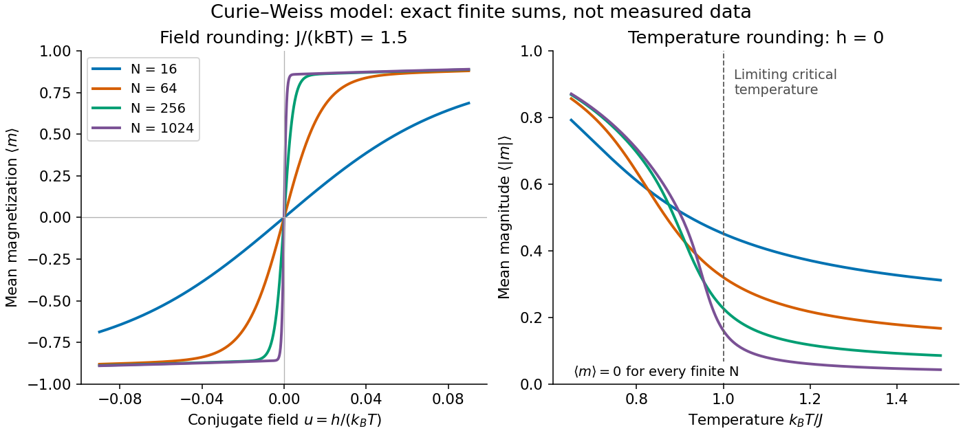
Every curve is computed from the finite partition function, without selecting one minimum of the Bragg-Williams free energy of the Ising model. The field panel holds $K=1.5$ fixed and shows increasingly rapid switching between opposite spin magnetizations. The temperature panel uses $u=0$: its nonzero $⟨|m|⟩$ measures the typical magnitude, while the mean spin magnetization stays zero. The reference $k_{B}T/J=1$ marks the limiting critical temperature, not a singular point of any finite curve.

A short limiting argument explains the field panel. Combining the binomial coefficient with its leading entropy gives a Helmholtz free energy per spin whose stationarity equation is $m=\tanh (Km+u)$. For $K>1$ and $u=0$ the two ordered minima have $m=\pm m_{\ast }$, where $m_{\ast }=\tanh (K{m}_{\ast })$. For large $N$ well below the critical temperature, their relative Boltzmann weight is approximately $e^{2Nu{m}_{\ast }}$, giving $⟨m⟩\approx m_{\ast }\tanh (Nu{m}_{\ast })$. Thus this two-peak approximation has a field width of order $1/(N{m}_{\ast })$ in $u$. It is not valid at the critical temperature, where the peaks merge; the figure uses the exact finite sum throughout.

At zero field and with spin inversion symmetry in its boundary conditions, a finite Ising model pairs every configuration with its spin-reversed configuration. Their equal Boltzmann weights force the expected value of its spin magnetization $m=N^{-1}{\sum }_i{s}_i$ to vanish. Below a model's ordering critical temperature, an arbitrarily small positive field can instead select the positive spontaneous magnetization if size is taken to infinity first:The distinction is the order of limits and the stated symmetric boundary conditions; plus boundary conditions already break spin inversion symmetry. A zero-field symmetric mixture of the two ordered states can retain zero mean spin magnetization even in the thermodynamic limit. Also, $⟨|m|⟩>0$ in a finite system is not by itself proof of spontaneous symmetry breaking.^[ref]

For finitely many microstates with finite energies $E_{\alpha }(h)$ that are real analytic functions of a real control $h$, the canonical partition function at $T>0$ is a finite positive sum:It and the resulting Helmholtz free energy are locally real analytic functions of $T$ and $h$. Hence such a finite Ising model has no literal nonanalytic equilibrium phase transition. A limit of these real analytic functions can nevertheless fail to be a real analytic function; the narrow but smooth crossover can become a sharp phase transition.^[ref]

Finite particle number alone is not the hypothesis of a finite sum. Classical phase space is continuous, and a system of quantum states can have infinitely many energy eigenvalues: its partition function requires convergence and local bounds that permit differentiation or an analytic extension of the integral or thermal trace. A divergent partition function, a singularly changed statistical Hamiltonian, or the zero-temperature limit falls outside the finite-positive-sum argument. Observing a steep change in a finite sample therefore motivates a limiting model; it does not measure an actual infinity.

A system call creating a child operating-system process from a parent. The Linux kernel documents copy-on-write for ordinary inherited private memory pages, with separate address spaces but shared open file descriptions for inherited file descriptors. ^[ref]

An NMDA receptor is an ionotropic receptor gating an ion channel with voltage-dependent magnesium block. This voltage dependence permits cooperative amplification when inputs produce sufficient local depolarization; calcium can also pass through the open channel.^[ref]

A dendritic spike is a regenerative local voltage event in a dendrite. Its effect at the soma depends on propagation and attenuation; local regeneration does not by itself establish a somatic action potential. It is an active mechanism beyond the passive dendritic cable.

A neuronal firing threshold specifies the condition for initiating an action potential. The leaky integrate-and-fire model uses a prescribed membrane potential $\vartheta$; real initiation involves active voltage-gated ion channels and depends on recent activity and recording site. A threshold drawn on a passive voltage trace is a comparison criterion, not a simulated action potential.

Temporal summation is overlap of responses to inputs arriving at different times. It can occur at one repeatedly activated synapse or across several synapses; it is not defined by reuse of a particular contact. For prescribed electric current inputs in a passive compartment, residual depolarization from earlier pulses changes the voltage reached by later pulses. The membrane time constant sets how rapidly that residual decays, while the duration of synaptic conductance and spatial filtering by a passive dendritic cable can add other timescales.

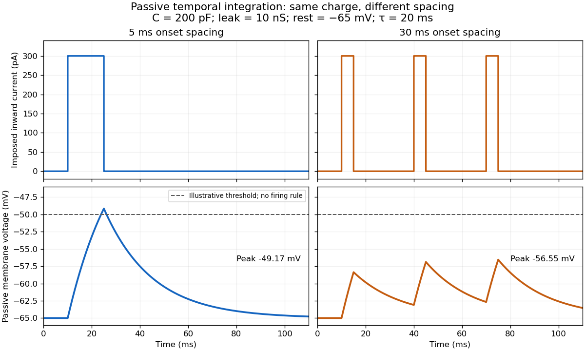
For the diagram, write $v=V-E_L$, choose inward-positive imposed electric current $I$, and use the ordinary differential equationA rectangular pulse of amplitude $I_0=300\mathrm{pA}$ and duration $d=5\mathrm{ms}$, starting from rest, ends withAfterwards its contribution decays as $A{e}^{-(t-d)/{\tau }_m}$. The superposition principle therefore gives, at the end of the third pulse with onset spacing $\Delta \ge d$,For $\Delta =5\mathrm{ms}$ this is $15.829\mathrm{mV}$, so the peak membrane potential is $-49.171\mathrm{mV}$. For $\Delta =30\mathrm{ms}$ it is $8.447\mathrm{mV}$, giving $-56.553\mathrm{mV}$. Both protocols inject $3I_{0}d=4.5\mathrm{pC}$ of electric charge; equal charge does not imply equal peak voltage because the leak drains charge while it is delivered.

In the adjacent-pulse case, the illustrative neuronal firing threshold $-50\mathrm{mV}$ is crossed at $10+20\log 2\approx 23.863\mathrm{ms}$. A leaky integrate-and-fire model would emit its first event there and reset, so its later trajectory would differ from the passive diagram. The widely spaced train never reaches that threshold. Thus changing input timing alone can change whether an event occurs. A real neuron's neuronal firing threshold is also state-dependent, and synaptic conductance pulses are not prescribed electric current pulses.^[ref]

Measured responses to repeated presynaptic action potentials may also change through synaptic plasticity. A larger second response can therefore reflect a stronger second input as well as residual postsynaptic voltage. To isolate passive temporal summation, compare known injected electric current waveforms with their single-pulse responses under stable recording conditions; to test actual synapses, measure whether input efficacy changes. These are proposed discriminating comparisons, not additional controls claimed for the slice experiment.^[ref]

Spatial summation combines inputs arriving at different synapses. Location matters because a dendrite has axial electrical resistance and leaky membrane capacitance: a local synaptic potential need not arrive at the soma with its original amplitude or time course. A passive dendritic cable makes this attenuation explicit. The superposition principle applies to fixed electric current inputs in a linear passive model, but adding synaptic conductances changes the model's coefficients. Compare voltage changes relative to the same baseline, rather than adding absolute membrane potentials.

A motivating experiment. A 2004 study used $300$–$350\mu \mathrm{m}$ cortical slices from $18$–$28$-day-old rats at $35$–$36{}^{\circ }\mathrm{C}$. Somatic whole-cell recordings measured EPSPs in layer-5 pyramidal neurons. Two fine stimulating electrodes were positioned beside imaged dendrites; calcium-sensitive dye localized activation. Each site was stimulated alone, then both together, usually with paired pulses $20\mathrm{ms}$ apart. Comparing the combined voltage trace with the sum of individual changes tested the summation rule. Nearby inputs on one branch showed strong amplification at intermediate strengths; inputs on different branches were approximately linear.^[ref]

Blocking both excitatory receptor classes eliminated voltage and calcium responses, checking against direct electrical activation. NMDA receptor blockers eliminated or markedly reduced amplification; comparisons with inhibition intact and blocked addressed inhibitory contributions. These controls support local active integration. Passing axons could still recruit unintended synapses; somatic voltage does not measure every local membrane potential. The study tested subthreshold slice responses and pairs of branches, not arbitrary activity in an intact brain.^[ref]

A synaptic potential is a postsynaptic change in membrane potential caused by activity at a synapse. Unlike the regenerative action potential, a passive synaptic potential is graded: its size depends on input strength, the initial membrane potential and the receiving cell membrane's properties. Local voltage changes can decay before reaching the soma; their timing and overlap help determine whether an action potential follows. See Ion Channels and the Electrical Properties of Membranes.

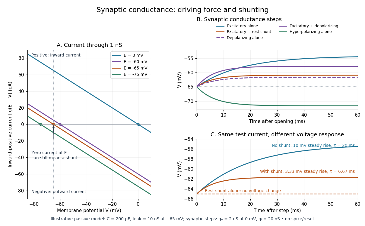
Depolarization means that the interior becomes less negative relative to the exterior; hyperpolarization means that it becomes more negative. Excitation and inhibition instead describe whether an input promotes or opposes postsynaptic action potential generation. An inhibitory postsynaptic potential can be depolarizing, and shunting inhibition can occur with no voltage change at rest. The receptor, permeating ions, ionic gradients and reversal potential matter. See Purves and colleagues: excitation, inhibition and depolarizing inhibition.

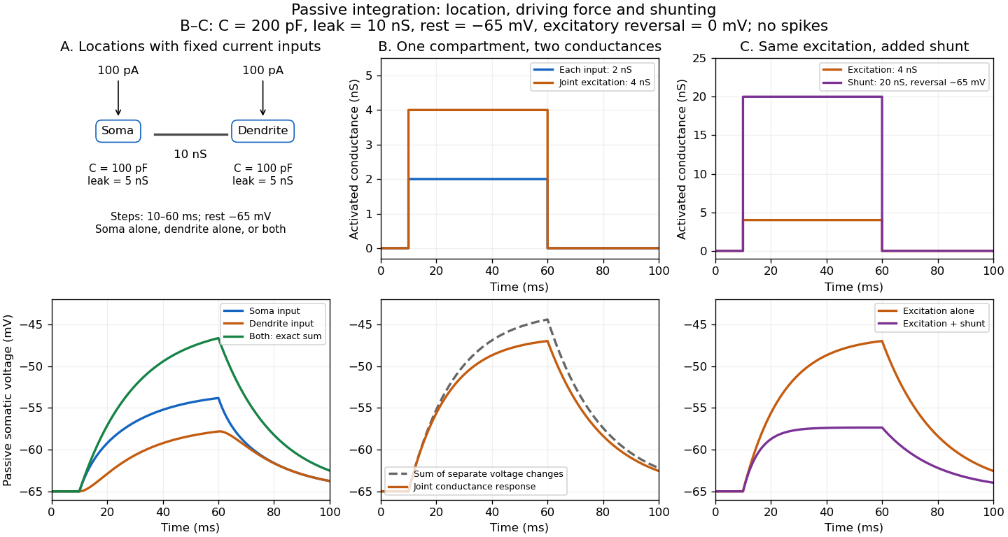
A worked passive model treats the receiving membrane as one compartment with capacitance $C>0$, leak conductance $g_L>0$, and activated synaptic conductances $g_e,g_i\ge 0$:All electric currents are inward-positive. Each term $g(E-V)$ vanishes at its reversal potential $E$; $\mathrm{nS}\times \mathrm{mV}=\mathrm{pA}$. With constant parameters, the ordinary differential equation hasHere $G$ is total conductance, $1/G$ is effective electrical resistance, $V_{\infty }$ is the steady state and $\tau$ the time constant. Without imposed electric current, $V_{\infty }$ is a conductance-weighted average of the reversal potentials. This approximation omits spatial structure, changing ionic gradients and active voltage-gated ion channels; it calculates passive voltage responses, not actual action potential waveforms. See 3.1 Synapses for the mechanism behind the terms; the inward-positive convention here reverses that source's synaptic-current sign.

Take the same illustrative leak and capacitance as under shunting inhibition, start at $V(0)=-65\mathrm{mV}$ and set $I_{\mathrm{ext}}=0$. Opening $g_e=2\mathrm{nS}$ with $E_e=0\mathrm{mV}$ gives $V_{\infty }=-650/12\simeq -54.167\mathrm{mV}$ and $\tau \simeq 16.667\mathrm{ms}$. Its initial inward electric current is $2(0+65)=130\mathrm{pA}$. Adding $g_i=20\mathrm{nS}$ with $E_i=-65\mathrm{mV}$ changes $V_{\infty }$ to $(-650-1300)/32=-60.9375\mathrm{mV}$ and $\tau =6.25\mathrm{ms}$. This is shunting inhibition of the same excitatory drive.

For comparison, $g_i=20\mathrm{nS}$ with $E_i=-75\mathrm{mV}$ alone gives $V_{\infty }\simeq -71.667\mathrm{mV}$: hyperpolarization. With $E_i=-60\mathrm{mV}$ instead, it alone gives $V_{\infty }\simeq -61.667\mathrm{mV}$: depolarization. Yet adding this depolarizing conductance to the $g_e=2\mathrm{nS}$ excitatory drive lowers that drive's $V_{\infty }$ from $-54.167$ to $(-650-1200)/32=-57.8125\mathrm{mV}$. At an illustrative firing threshold $V=-50\mathrm{mV}$, its electric current is $20(-60+50)=-200\mathrm{pA}$, opposing threshold approach. The combined trace initially rises faster than the excitatory drive alone, before settling below it. Thus the sign of a voltage change at rest alone does not determine excitation or inhibition; a claim about firing must specify input strength, timing and the neuron's state.

An electrical synapse passes ionic electric current directly between neurons through gap junctions, whose paired channels connect the two cytoplasms. It does not require synaptic vesicle release and postsynaptic neurotransmitter binding. Transmission across the junction is very fast; the receiving cell membrane's capacitance and other conductances still determine its voltage response. Electrical coupling can coordinate the timing of activity across neurons. See Purves and colleagues: electrical synapses and gap junctions.

For a passive junction with constant conductance $g_j$, the inward electric current into cell 2 iswhere each $V_k$ is the cell's membrane potential, measured against a common extracellular reference. Taking $g_j=2\mathrm{nS}$, $V_1=-55\mathrm{mV}$ and $V_2=-65\mathrm{mV}$ gives $20\mathrm{pA}$ into cell 2 and the equal opposite electric current into cell 1. Exchanging the voltages reverses the electric current. Both depolarization and hyperpolarization can therefore be transmitted; an electrical synapse is not inherently an excitatory connection.

Many electrical synapses conduct in both directions, but this does not guarantee equal voltage responses: the cells can have different effective electrical resistance and capacitance. Some junctions rectify, meaning they conduct preferentially in one direction, so the constant-$g_j$ formula is insufficient. A concrete molecular example is the original study ^[ref]. Bidirectionality is thus a common property with important qualifications, rather than part of the definition.

A chemical synapse transmits a signal by releasing neurotransmitter from a presynaptic neuron to act on postsynaptic receptors across a synaptic cleft. The two cell membranes remain separate. A typical fast transmission sequence is:

See Chemical Synapses and 3.1 Synapses. The fast pathway uses synaptic vesicles prepared near release sites; it does not require a distant synaptic vesicle to travel across the terminal after every action potential. See Basic Neurochemistry: calcium entry and vesicles at release sites. Some chemical synapses release neurotransmitter in response to graded presynaptic membrane potential changes rather than action potentials.

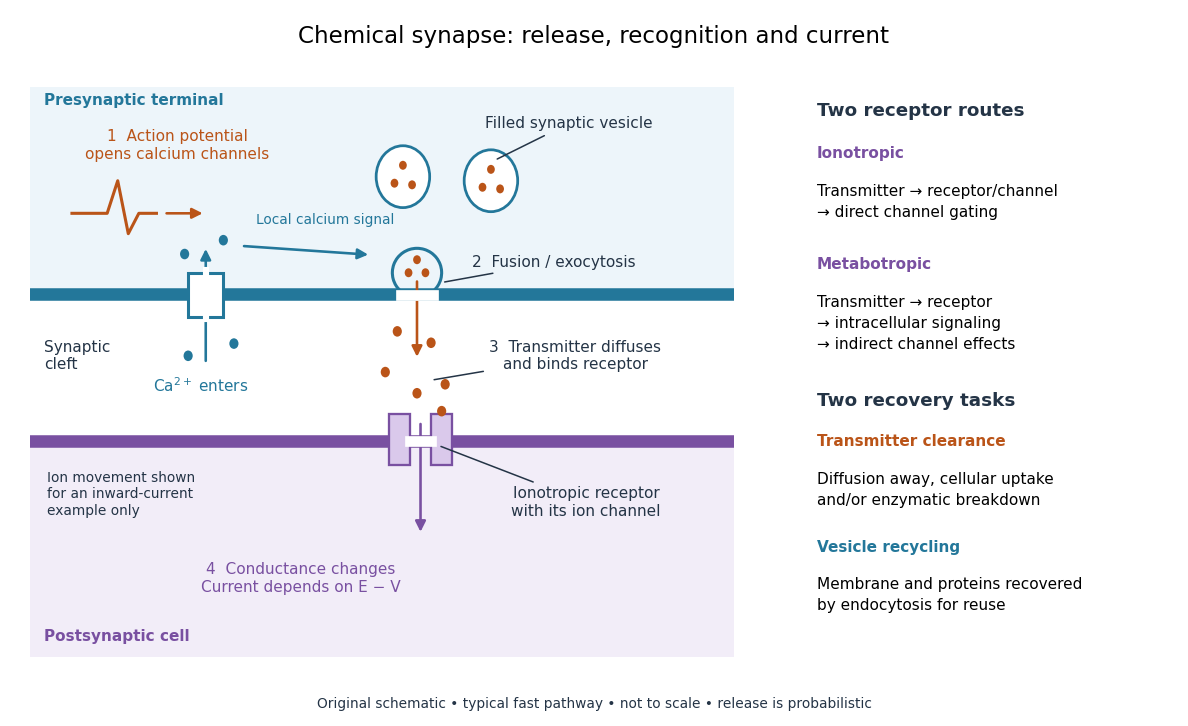
Neurotransmitter clearance limits how long released neurotransmitter remains available. Depending on the neurotransmitter and location, diffusion away, uptake through membrane transport proteins into the sending or neighboring biological cells, and breakdown by enzymes contribute. Receptor binding and unbinding also affect response duration. Recovering synaptic vesicle membrane is a separate recycling task; uptake of released neurotransmitter is not the return of an intact synaptic vesicle. See General Principles of Cell Communication.

This electrical-to-chemical-to-electrical sequence offers several places to adjust a signal: synaptic release probability, receptor availability and neurotransmitter clearance can change its strength or duration. It helps explain why synaptic plasticity can modify communication between neurons, and why an arriving action potential need not cause a postsynaptic action potential.

Otto Loewi's 1936 Nobel lecture describes his 1921 experiment: fluid from a frog heart whose nerves had been stimulated produced the corresponding response when transferred to another heart. The transferable substance established chemical mediation in that preparation. This was evidence for released chemical signaling, not yet an identification of synaptic vesicle fusion and not a claim that every synapse is chemical. See Loewi, The Chemical Transmission of Nerve Action, Nobel lecture, 12 December 1936.

A chemical signal released by a neuron that changes a target cell's activity through its receptors. Its effect depends on the receptor and ionic mechanism rather than being intrinsically excitatory or inhibitory in every context.

Changes in synaptic efficacy over time. Activity-dependent plasticity can support learning and development, but also requires constraints to prevent unbounded growth or competition in simplified models.

Here $p_{\alpha }$ is a product of power-sum symmetric functions and $z_{\alpha }={\prod }_r{r}^{m_r}{m}_r!$ for part multiplicities $m_r$. The Frobenius characteristic map identifies this product with the ordinary character inner product. Schur functions are orthonormal, and the adjoint of multiplication by $p_k$ is $k\partial /\partial p_k$. These properties turn a power-sum multiplication formula into the Murnaghan–Nakayama rule.

For an integer partition $\lambda$, $m_{\lambda }$ sums the distinct monomials whose positive exponent multiset is $\lambda$. No multiplicity is attached to repeated parts. The functions of fixed total degree form a basis of the symmetric functions of that degree, since finite variable permutations identify precisely these monomial orbits.

The Fundamental theorem of symmetric polynomials gives freely generated elementary functions, so sending each $e_r$ to $h_r$ defines an algebra homomorphism. For $E(t)=\sum e_r{t}^r$ and $H(t)=\sum h_r{t}^r$, $E(-t)H(t)=1$. Applying the homomorphism shows $\omega (H(t))=E(t)$, hence ${\omega }^2=1$. Taking logarithms of $H$ gives the displayed action on power sums. It preserves the Hall inner product of symmetric functions because each power-sum basis vector acquires only a sign.