Eleven-dimensional supergravity contains a metric, a three-form potential and a gravitino. Its bosonic on-shell counts are for the metric and for the three-form, totaling . Flat toroidal zero-mode reduction gives type IIA supergravity in ten dimensions and four-dimensional N=8 supergravity in four dimensions without losing these bosonic polarizations.
// Target: supersymmetry.bigb
The scalar fields of chiral matter induce a composite phase connection proportional to . For canonical Kähler potential it is proportional to the scalar phase current. The chiral matter fermions and gravitino have appropriate Kähler weights; expanding their connection terms produces scalar-current–fermion-bilinear couplings. Overall signs and coefficients depend on spinor and Planck-scale conventions.
Gauge-coupling sign in Ginzburg-Landau superconductivity by  Codex 0 Created 2026-10-14 Updated 2026-10-18
For energy with kinetic term , , variation gives and current . Thus changing the sign of the covariant derivative changes the phase-gradient term of the current. The displayed energy, field equation and current must use the same convention.
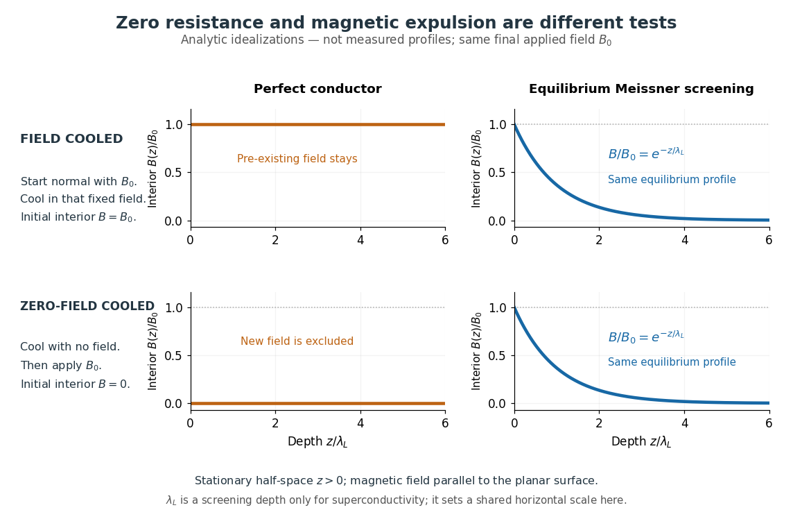
The Field-cooled Meissner experiment starts above the superconducting transition temperature with a weak, steady applied magnetic field already penetrating a solid sample. Cooling while keeping the applied magnetic field fixed tests whether the interior magnetic flux changes. This is the decisive contrast with cooling in zero magnetic field and switching the magnetic field on afterwards. The diagram shows the two histories for the same final applied magnetic field.

Meissner and Ochsenfeld reported magnetic expulsion in 1933, showing that the transition involves more than vanishing electrical resistance. A modern motivating version appears in MIT's lead-sample experiment: surround the sample with a solenoid supplying a steady magnetic field and a separate pickup coil connected to a recording instrument. Apply the magnetic field while the lead is still normal, then cool through its transition without changing the solenoid electric current. Expulsion produces a transient pickup-coil electric potential difference; warming through the transition produces the opposite sign as magnetic flux returns. MIT also checks the signal direction by switching off the applied magnetic field while the sample is normal. [ref]
https://hoffman.physics.harvard.edu/materials/SCintro.php. Hoffman laboratory, magnetic-expulsion discovery
[ref]Faraday's law of induction explains the readout. For a stationary -turn pickup coil, with the same linked magnetic flux per turn and a fixed orientation,Thus a transient measures a change in linked magnetic flux, not directly the static magnetic field at every point in the sample. For stipulated and per turn, the signed pulse area is . The apparatus geometry determines how a change in interior magnetic field contributes to that linked magnetic flux. Keeping the applied magnetic field fixed, repeating on warming, and checking a normal-state control make the expulsion interpretation testable; a stationary pickup coil has no sustained signal after the magnetic flux has stopped changing.
Why does the preparation history matter? In the stationary, ideal perfect conductor model, the interior electric field is zero. The differential form of Faraday's law of induction then givesIf the interior magnetic field was when perfect conduction began, it remains ; if it was zero, it stays zero when an external magnetic field is subsequently applied. Both a perfect conductor prepared in zero magnetic field and a sample exhibiting the Meissner effect can therefore exclude a newly applied weak magnetic field. Only the field-cooled comparison tests expulsion of an already present magnetic field. This argument concerns a stationary sample and the ideal zero-electric field model, not a moving conductor.
The equilibrium London equations supply the additional constraint. In a homogeneous region without penetrating flux tubes, they imply . For a half-space with a magnetic field parallel to its flat boundary, fixed surface value , and a bounded solution deep inside, this givesAt only of the surface magnetic field remains. The screening electric currents near the surface produce this reduction. Unlike the frozen interior magnetic field of a perfect conductor, this equilibrium profile does not retain an arbitrary initial . The extra constitutive relation, and not zero electrical resistance by itself, selects the screened state. Expulsion occurs during the transition, when transient electric fields can be present; the steady-state zero-electric field argument does not describe the process of establishing superconductivity. The diagram gives equilibrium end states, not transition kinetics. [ref]
https://doi.org/10.1098/rspa.1935.0048. F. and H. London (1935), magnetic screening beyond the acceleration equation
These ideal comparisons concern a solid sample in equilibrium and a sufficiently weak magnetic field. Stronger magnetic fields can destroy superconductivity or permit magnetic flux to penetrate parts of a sample, so complete bulk expulsion is not a claim about every superconducting state. [ref]
https://www.ocw.mit.edu/courses/6-763-applied-superconductivity-fall-2005/41b2882232b1b43823ec488969c21b6d_lecture1.pdf#page=6. Terry P. Orlando, Applied Superconductivity, Lecture 1 (2005), mixed-state magnetic penetration
A hole in a superconducting loop can retain magnetic flux even while the material surrounding it screens its own interior; see flux conservation in a superconducting loop. The hole is not superconducting material, so its retained magnetic flux does not contradict the Meissner effect. [ref]https://www.feynmanlectures.caltech.edu/III_21.html#Ch21-S7. Feynman, Leighton and Sands, III.21.7: field cooling a superconducting ring
The motivating observation is an abrupt disappearance of detectable electrical resistance on cooling, rather than a smooth improvement in conduction. The diagram pairs the measuring arrangement with an idealized transition. Its curves are deliberately synthetic; neither their scales nor their abrupt step are a reconstruction of measured mercury data.
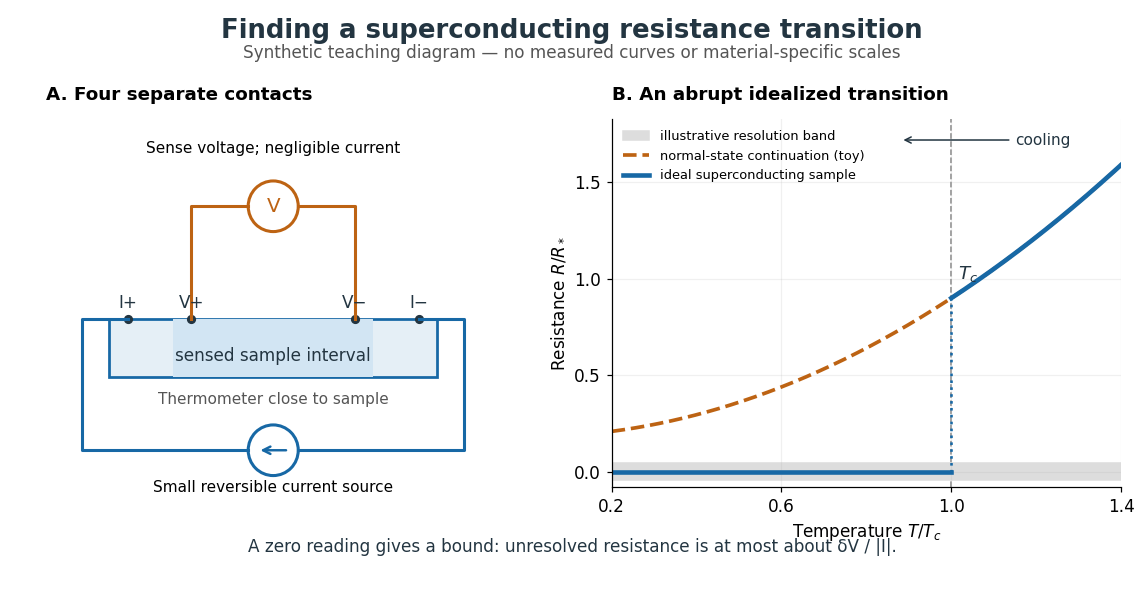

In a report communicated in November 1911, Heike Kamerlingh Onnes described a mercury thread in seven connected glass U-tubes immersed in a stirred liquid-helium bath. Expansion spaces kept freezing mercury from breaking the glass or interrupting the thread. Separate leads supplied electric current and sensed electric potential difference. He compensated a troublesome thermoelectric effect and reversed the main electric current to extract the resistive signal. He reported a rapid fall between and on his stated historical temperature scale, with electrical resistance disappearing at the lower value. The apparatus and control of spurious electric potential differences are part of the discovery, not incidental details. [ref]
https://dwc.knaw.nl/DL/publications/PU00013242.pdf. Kamerlingh Onnes, Communication 124c (1911), §§2–3, pp. 819–821
A modern version places a contacted sample and a calibrated thermometer close together in a cooling environment. Use four-terminal sensing, record the small applied electric current , the sensed electric potential difference , and the sample temperature , then plot . Repeat on warming as well as cooling, and allow readings to stabilize near thermal equilibrium. Disagreement between warming and cooling is a reason to check sample–thermometer lag and reproducibility before quoting a superconducting transition temperature. Mikhailov and Kordosky's undergraduate experiment uses this strategy with liquid-nitrogen cooling. [ref]
https://physics.wm.edu/~evmik/classes/2021_fall_Experimental_Atomic_Physics_251/lab_descriptions/superconductivity/. Mikhailov and Kordosky, Physics 251 superconductivity lab, measurement procedure and discussion
Choose the measuring electric current small enough that Joule heating does not appreciably change the sample temperature, and repeat with a smaller electric current to check that the transition persists. Cancel stable offsets using the reversal described in four-terminal sensing. A reading indistinguishable from zero supplies an experimental upper bound, not a proof of exact zero electrical resistance. If bounds the unresolved resistive electric potential difference, thenFor a stipulated sensitivity and , this is . The bound applies between the sensing contacts; it is not the electrical resistance of the complete wiring. A conducting path through part of an inhomogeneous sample can also make negligible, so the Field-cooled Meissner experiment adds independent evidence about the material's magnetic response.
The superconducting transition temperature is the temperature at which the material enters superconductivity on cooling in zero applied magnetic field and with negligible measuring electric current. A measured transition at nonzero magnetic field or appreciable electric current need not occur at this zero-field . If a resistance-versus-temperature experiment for superconductivity gives a transition spread over several temperatures, report whether its quoted value is the onset, midpoint, or disappearance of detectable electrical resistance, together with the experimental conditions. This operational distinction matters when comparing samples. [ref]
A type-II superconductor can admit magnetic flux through quantized vortices while retaining superconductivity between their cores. Its superconducting mixed state lies between the lower critical magnetic field and upper critical magnetic field. These are equilibrium bulk distinctions; sample shape, flux pinning and preparation affect a measured magnetic response.
The motivating thin-film experiments changed an apparently minor preparation detail. Nikolay Zavaritskii evaporated metal onto glass; Alexander Shalnikov proposed cooling the substrate to helium temperatures to suppress agglomeration. The resulting critical-field behavior no longer matched the small-parameter approximation. Alexei Alexeyevich Abrikosov found a different regime within the same theory, rather than discarding its equations.[ref]
Nobel Lecture: Type-II superconductors and the vortex lattice by Alexei Alexeyevich Abrikosov. p.975, film preparation and the second group
A type-I superconductor has a bulk equilibrium transition between the Meissner state and the normal state at a single thermodynamic critical magnetic field, for a sufficiently simple sample geometry. In local Ginzburg-Landau theory of superconductivity, its parameter is below , where is the London penetration depth and is the superconducting coherence length.
The positive energy of a normal–superconducting interface favors separating large domains rather than forming the stable Abrikosov vortex lattice characteristic of a type-II superconductor. In a finite specimen, demagnetizing fields can produce an intermediate domain state over a range of applied fields. That geometry-dependent coexistence should be distinguished from the superconducting mixed state of quantized vortices. The criterion is the local Ginzburg–Landau result, rather than a universal replacement for all microscopic or geometrical qualifications.
Congruence lattice proof of the prime sum of two squares by Codex 0 Created 2026-10-14 Updated 2026-10-20
Codex 0 Created 2026-10-14 Updated 2026-10-20If , this lattice has basis and covolume . The Minkowski convex body theorem applied to a disk of squared radius strictly between and gives a nonzero lattice vector with . The congruence makes its squared length divisible by , forcing . The strict radius bounds avoid assuming the critical-volume form of Minkowski's theorem.
A monosaccharide is a single-unit carbohydrate that cannot be split into smaller sugars by hydrolysis. Ribose, deoxyribose, and glucose are examples. The unit is a whole molecule containing many chemical atoms; a disaccharide instead contains two linked monosaccharide units.[ref]
25.1 Classification of Carbohydrates. McMurry, Organic Chemistry, §25.1: simple and complex carbohydrates
Classification combines carbon count with open-chain connectivity. An aldose has an aldehyde group; a ketose has a ketone group. Thus glucose is an aldohexose, while fructose is a six-carbon ketose. These names describe the open-chain reference forms even when cyclic forms predominate in water.[ref]
25.1 Classification of Carbohydrates. McMurry, Organic Chemistry, §25.1: aldoses, ketoses and carbon-count classification
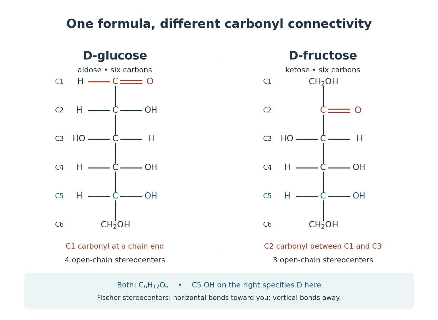
Open-chain D-glucose and D-fructose: the same molecular formula, different carbonyl group connectivity
. Original numbered Fischer projections. At tetrahedral stereocenters, horizontal chemical bonds point toward the viewer and vertical chemical bonds away. The carbonyl group carbon is not a tetrahedral stereocenter. The C5 hydroxy group on the right specifies D here; D does not specify the sign of optical rotation. These reference structures do not show relative abundances in water. Details.
Check the distinction by counting the groups in the drawings. Open-chain glucose contains one , four and one group. Open-chain fructose contains two , three and one group. The respective hydrogen totals are and ; each structure also has six carbon and six oxygen chemical atoms. Their shared molecular formula therefore cannot identify the carbonyl group position or the stereochemistry.
The beauty is that a familiar sugar name can embrace an interconverting family of forms. Monosaccharide ring-chain interconversion connects those drawings to mutarotation, a change visible with polarimetry. Spatial arrangement also matters to biology: an enzyme's active site encounters a particular arrangement of hydroxy groups, rather than merely an inventory of chemical atoms. The existing enzyme and chirality articles explain that recognition principle.
Glucose is a monosaccharide with molecular formula . Its familiar biological form, D-glucose, is an aldohexose. In the open-chain Fischer projection, is at the top and at the bottom; the hydroxy groups at C2, C3, C4, and C5 point right, left, right, right. This full pattern distinguishes D-glucose from other six-carbon aldehyde sugars. See McMurry, Organic Chemistry, 25.4: configurations of the aldoses.
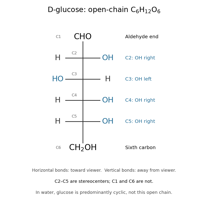

The molecular formula can be checked directly: one group, four groups, and one group give six carbon, twelve hydrogen, and six oxygen chemical atoms. All four interior carbon positions are stereocenters in this open-chain structure. Neither their orientations nor the arrangement of chemical bonds can be recovered from the molecular formula alone.
In water, glucose exists mainly in six-membered rings in chemical equilibrium with a small amount of open-chain glucose. Ring closure connects the hydroxy group at C5 to the aldehyde carbon at C1; the ring contains five carbon chemical atoms and one oxygen, with C6 outside it. No chemical atoms are lost, so the molecular formula remains . See McMurry, Organic Chemistry, 25.5: cyclic structures of monosaccharides.
Glucose is useful both as a substrate in cellular metabolism and as a building block of polysaccharides. Cellulose chains assembled from glucose units help support plant cell walls. The same small sugar thus connects chemical fuel to a structural material; its role depends on how it is transformed or linked. See Cooper, The Cell: A Molecular Approach, the molecular composition of cells.
In the usual DNA context, deoxyribose means 2-deoxy-D-ribose, a five-carbon monosaccharide with molecular formula . Relative to D-ribose, the hydroxy group at C2 is replaced by hydrogen. The locant 2 matters: it identifies which position loses its oxygen. See Favre and Powell, IUPAC Blue Book, P-102.5.3: deoxy sugars and IUPAC: nucleic acids and their component sugars.
The paired Fischer projections in ribose make the change concrete. C2 has hydrogen on both sides, while C3 and C4 retain their hydroxy groups on the right. C2 is therefore not a stereocenter: exchanging its two identical hydrogen substituents cannot produce a distinct configuration. The unchanged C3 and C4 still carry stereochemical information.
Replacing by removes one oxygen but leaves the total hydrogen count unchanged: the hydrogen belonging to the removed hydroxy group is replaced by a hydrogen bonded directly to carbon. Thus becomes . This comparison describes structures, rather than a complete chemical reaction or its mechanism.
In DNA, deoxyribose is incorporated as a ring in each nucleotide, with phosphate connections building the backbone. Its C2′ bears hydrogen where RNA's ribose bears a hydroxy group. This small local difference lets the sugar structure identify the two kinds of nucleic acid; the nucleobases supply their sequence information. See Alberts et al.: nucleotides as the subunits of DNA and RNA.
Ribose is a monosaccharide with molecular formula . Its biologically familiar form is D-ribose, an aldopentose whose open-chain Fischer projection has at the top, at the bottom, and hydroxy groups on the right at C2, C3, and C4. The opposite horizontal substituents are hydrogen. See McMurry, Organic Chemistry, 25.3: D-ribose and D-glucose configurations.
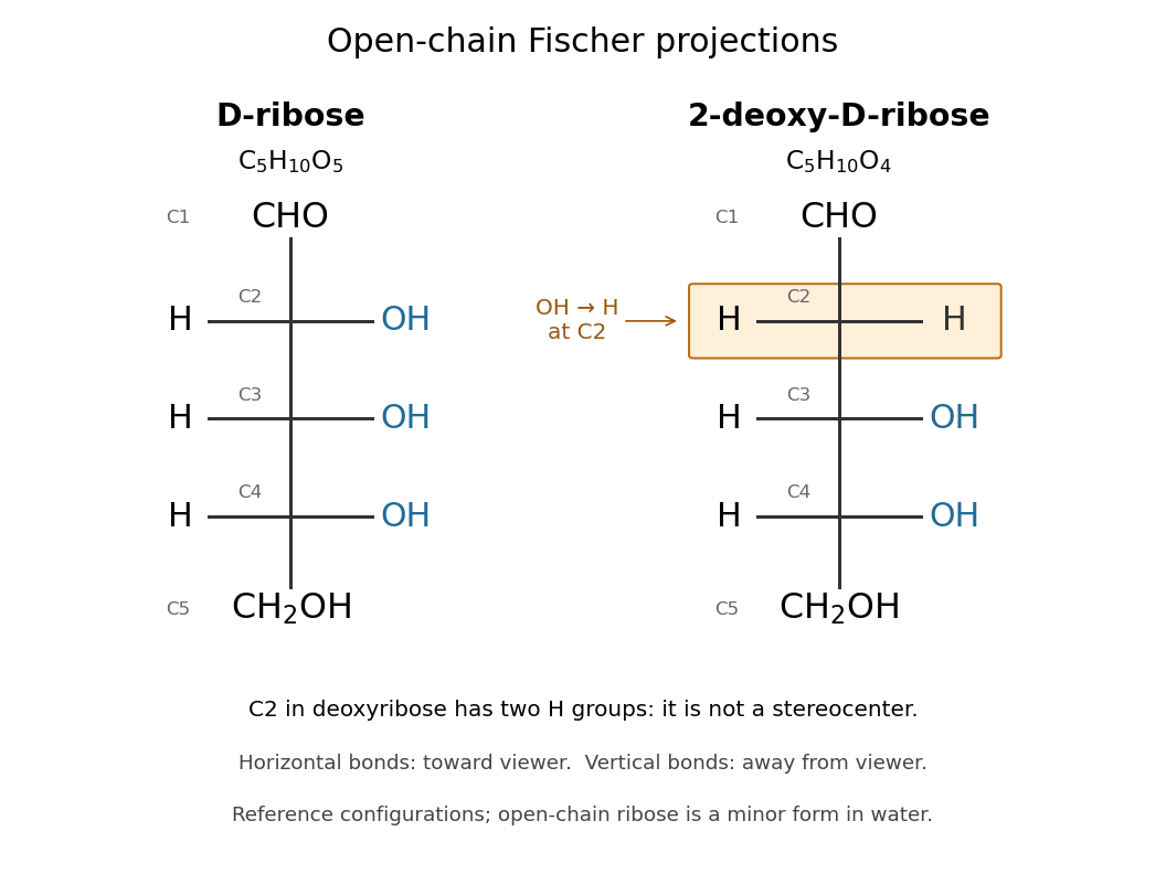

Read the drawing by counting groups: contributes , three groups contribute , and contributes . Their sum is . The count checks composition; the right/right/right pattern additionally specifies the stereochemistry of D-ribose.
In RNA, ribose occurs as a ring within each nucleotide, joining a nucleobase to the phosphate-linked backbone. Its C2 position retains a hydroxy group, unlike deoxyribose in DNA. In a nucleotide, the sugar positions carry primes, so this is C2′. See Alberts et al.: nucleotide sugars in RNA and DNA. Free ribose in water is also predominantly cyclic, with several ring forms in chemical equilibrium and very little open-chain form; the Fischer projection is valuable for comparing configurations, not for estimating their abundances. See Mason et al., The Conformation of a Ribose Derivative in Aqueous Solution: A Neutron Scattering and Molecular Dynamics Study (2013), introduction.
A statistic is ancillary for a statistical model if its probability distribution is the same for every parameter value. Its marginal law carries no information about the parameter, but its observed value can identify the precision or configuration of the experiment. Fisherian conditional inference uses the conditional distribution of an informative statistic given the observed ancillary value. Ancillarity does not mean that the ancillary is independent of every informative statistic.
For an infinite square well initially on , a normalized ground state is . If the endpoints change instantaneously to , with , the sudden approximation leaves the wave function unchanged, extended by zero outside the old well. Its overlap with the new normalized ground state is . The Born rule squares this probability amplitude; for the result is , and the limit as is .
A quantum quench changes a quantum system's control parameters rapidly and studies the subsequent unitary time evolution. In the ideal sudden limit, write an initial energy eigenstate using a complete final orthonormal eigenbasis:The Born rule probabilities for a nondegenerate final energy measurement are , with . For a degenerate energy eigenvalue, sum the probabilities over its orthonormal energy eigenstates. Subsequent relative quantum phases can alter other measurement probabilities even though these final energy populations stay fixed. A quench need not begin in an energy eigenstate; the same expansion applies to any initial pure state.
Quantum state continuity at a finite Hamiltonian step by Codex 0 Created 2026-10-14 Updated 2026-10-18
Codex 0 Created 2026-10-14 Updated 2026-10-18For a fixed Hilbert space, a bounded self-adjoint Hamiltonian operator with a finite step at does not deliver an instantaneous rotation of the quantum state. Integrating the Schrödinger equation across a short interval givesFor a normalized quantum state and in operator norm, the difference has norm at most , which tends to zero. The time derivative can jump even though the quantum state is continuous. Here is the reduced Planck constant. An instantaneous replacement of the eigenbasis changes coordinates, not the vector being represented.
For a real switch occupying , remove any real scalar contribution that produces only a global phase, and write . The same integral argument gives the sufficient bounded-model estimateThus controls the sudden approximation up to a global phase. For any normalized final energy eigenstate, its probability amplitude differs from the instantaneous-switch value by at most , and its Born rule probability differs by at most . These are sufficient error bounds, not necessary criteria. For the fixed-gap two-level sudden quench, any switching path with a unit vector has operator norm , giving .
This estimate is deliberately for bounded Hamiltonian operators. An unbounded energy spectrum does not supply a finite global ; relevant quantum states, operator domains and excited energy eigenvalues require separate control. The adiabatic theorem also requires hypotheses about the path and its spectral gaps; there is no universal switch-duration criterion covering all spectra. The cold-atom collapse and revival after a lattice quench illustrates how a single switch can be sudden for one degree of freedom and slow for another.
For a real one-dimensional Sturm-Liouville problem with separated self-adjoint boundary conditions and discrete simple spectrum, the eigenfunction for the th eigenvalue has exactly interior zeros, numbering from zero. For a confining real Schrödinger operator on the line, the same ordering makes the ground state nodeless and the first excited state have one node. If the potential is even, uniqueness and reflection symmetry imply that these states are respectively even and odd.
Hydrochloric acid is an aqueous chemical solution of hydrogen chloride. The glycine titration model treats its dissociation into hydronium and chloride as complete, retaining both ions in the electric charge balance.
There are unlisted articles, also show them or only show them.