Changing the number of hash buckets and reassigning stored records using the new bucket-index hash function. Amortized analysis of rebuilding and expected value bounds for subsequent lookup address different costs.
Rebuild the balanced example from load factor of a hash table with while keeping exactly the same twelve records. Under , keys retain their indices, whereas keys move from hash buckets to hash buckets . The new chain lengths are twelve ones followed by four zeros; . Copying the old eight chain heads and adding eight empty heads would leave those four moved keys unreachable by the new lookup rule.
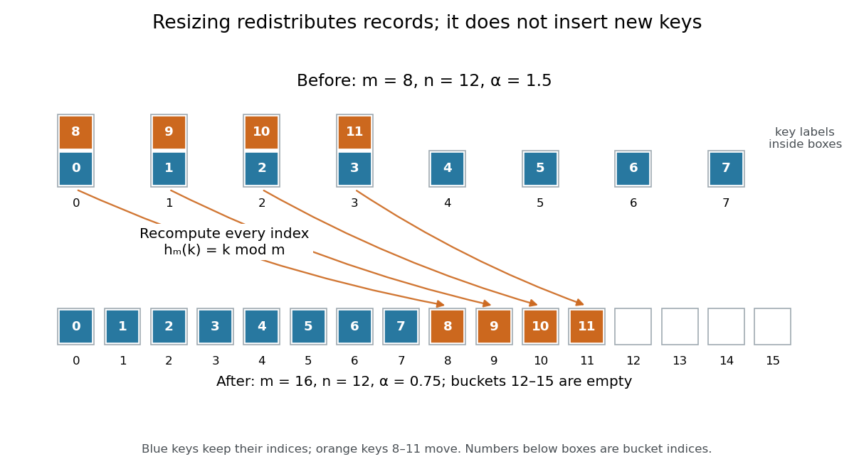
Hash table resizing from eight to sixteen hash buckets redistributes existing records
. Original modular arithmetic example for keys . Blue keys keep their indices; orange keys move because differs from . The record count stays twelve, and empty hash buckets still count towards capacity. Details.
For a short algorithm correctness outline, allocate the new array, visit every old record once, compute its new bucket index, and link it into that hash bucket. At every step, each transferred record is stored exactly once at the index prescribed by the new hash function. Finishing the visit therefore preserves every key-value association and makes the new lookup rule valid. Direct transfer can skip duplicate searches because the old one-value-per-key map already established distinct equivalence classes; rebuilding is not twelve new user insertions.
Under constant-cost hashing, linking and slot initialization, separate chaining rebuilding takes time complexity: initialize new heads, examine old heads, and transfer records. For doubling, , this is in Big O notation. It is when the resize policy makes proportional to , but an enormous mostly empty old array can make scanning its heads dominate. Growing capacity can lower without shortening a particular chain: the concentrated keys all remain in hash bucket after growth from eight to sixteen.
For an insertion-only sequence starting empty, choose initial capacity and double before a genuinely new key would make . The first three growths occur before inserting records and transfer existing records. If distinct records are inserted, the transfer count is . More generally, the transferred old capacities form a geometric series; if the last is , their sum is . Initializing and scanning these geometrically growing arrays also costs in total, giving amortized rebuilding overhead per insertion. A triggering insertion still pays for its whole rebuild.[ref]
Lecture 9: Hashing II. 6.006 Introduction to Algorithms, Fall 2011 by Massachusetts Institute of Technology, 6.006 course staff; p. 2, Rehashing, How fast to grow?, and Amortized Analysis
The illustrative twelve-record resize above is an explicitly requested rebuild, not a growth triggered by this threshold policy. Checking for an equal key before growing also prevents a value replacement from triggering unnecessary growth. To combine resizing overhead with expected constant insertion time complexity, separately impose the collision and constant-cost assumptions in load factor of a hash table. Amortized analysis distributes rebuilding costs over operations; it does not randomize a poor hash function or bound a single operation's latency. With deletions, separate the grow and shrink thresholds; for example, growing when full and halving at one-quarter live occupancy leaves room for many operations between opposite rebuilds.[ref]
Lecture 9: Hashing II. 6.006 Introduction to Algorithms, Fall 2011 by Massachusetts Institute of Technology, 6.006 course staff; p. 3, Back to Hashing and Delete: halving when n reaches m/4
// Target: computer-science.bigb
The number of stored records divided by the number of hash buckets. For separate chaining, this is the mean chain length over all hash buckets, including empty ones.
Consider two original separate chaining placements using the deterministic hash function on nonnegative integer keys. With , keys give the balanced chain lengths . Instead, keys all select hash bucket , giving . Both store records, so both have . The maximum chain lengths are and . These are constructed placements, not measured workloads.
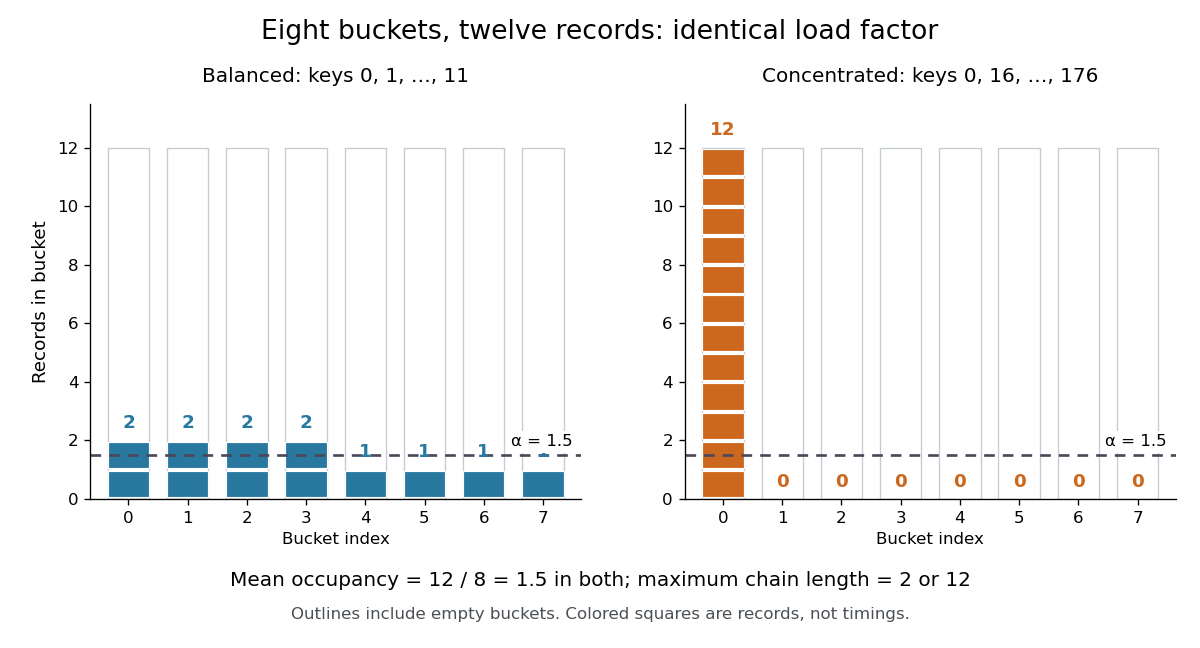
The same hash table load factor permits balanced and concentrated hash bucket occupancies
. Both original examples use eight hash buckets and twelve distinct integer keys. Every outlined column counts towards , including empty ones; each colored square represents one record. The dashed line marks the arithmetic mean , not the maximum chain length. Details.
For an absent query, separate chaining inspects every record in the selected hash bucket. Key selects hash bucket in both examples but is stored in neither, so it takes two key equality comparisons in the balanced placement and twelve in the concentrated placement. Key selects hash bucket and instead takes one comparison in the balanced placement and zero in the concentrated placement. If an absent query's bucket index has the uniform distribution on a finite set of eight indices, its mean comparison count is in either fixed placement. That average does not limit the cost of a particular query.
For successful lookups, suppose each of the twelve stored keys is queried with equal probability, with fixed chain order and no rearrangement on access. A chain of length contributes comparison counts , irrespective of its order. ThusThe balanced placement gives comparisons; the concentrated placement gives . Even this average depends on more than : concentration appears through the squared chain lengths. These exact counts exclude computing the hash function, locating the hash bucket, and allocating records. Elapsed lookup time also depends on the cost of key equality, key length, and memory access latency; alone specifies none of them.
The expected time complexity bound for separate chaining needs a probabilistic assumption. Fix distinct stored keys and a query independently of the random choice of hash function, and require for every unequal pair, where is a constant independent of . With constant-cost hashing, array access and key equality, this suffices. The authored chaining analysis cited here uses this pairwise-collision argument; its multiplicative construction has , rather than the of simple uniform hashing.[ref]
5.1 ChainedHashTable: Hashing with Chaining. Open Data Structures: An Introduction by Pat Morin; section 5.1.1, Lemma 5.1 and the indicator-variable proof of Lemma 5.2
For the proof outline, let be the indicator random variable that stored key shares an absent query 's hash bucket. By linearity of expectation,A present query's full chain contains itself plus at most other records, giving . Stopping at the match can only improve this bound. Full independence is unnecessary for this calculation, but fixed known hash functions and keys chosen adaptively to collide are outside the stated assumption. Keeping bounded then controls expected lookup work, while the concentrated example still explains why it gives no worst-case guarantee.
For the balanced twelve-record map,
put(3,new_value) replaces a value, so and remain unchanged. An absent key such as instead adds a thirteenth record, giving if capacity stays fixed. Under a policy that stores every repeated-key record separately, another record with key would also increase ; all equal-key records necessarily share a hash bucket when the hash function respects key equality. State the map policy before interpreting the count.The appeal of the hash table load factor is that one number helps tune a space-versus-search tradeoff: more hash buckets require more array storage and can reduce expected search work under the stated assumptions. The actual chain lengths and query choices still matter.
In open addressing, counts record slots and counts live records, so . A policy retaining at least one genuinely empty slot requires ; being below one is not itself a speed guarantee. For deletion using a tombstone in open addressing, also track , the number of marked slots: counts slots that cannot terminate an unsuccessful probe. For example, gives live occupancy but nonempty-or-marked occupancy . These ratios answer different questions.[ref]
5.2 LinearHashTable: Linear Probing. Open Data Structures: An Introduction by Pat Morin; section 5.2, three entry types, counters n and q, and find stopping at nil
The equivalence relation used to decide whether two keys name the same record. A hash function must respect key equality; a hash collision does not establish key equality.
The choice of key equality is part of the map's meaning. In the one-value-per-key policy of hash table, one record represents each stored equivalence class of keys:
put(k,v) updates an existing equal key and adds a record only if no equal key is present. A collection that deliberately retains repeated equal keys has a different policy; its load count must count those extra records too. Repeated calls and distinct stored records are different quantities.[ref]Lecture 8: Hashing I. 6.006 Introduction to Algorithms, Fall 2011 by Massachusetts Institute of Technology, 6.006 course staff; p. 1, Dictionary Problem: distinct keys or replacement on repeated insertion
For an original example, restrict keys to two-letter strings using letters
A through Z or a through z. Declare two keys equal when replacing every uppercase letter by its lowercase counterpart gives the same string. Assign each letter its position in the alphabet, ignoring case, and define the bucket-index hash function as the sum of the two positions modulo , using modular arithmetic. Then AB and ab are equal keys and both select hash bucket . Key ba also selects hash bucket because , but is unequal to ab: order still matters. Starting empty, put(AB,7), put(ab,9), put(ba,4) leave two records, with values for the ab equivalence class and for ba; the hash table load factor is , not .The compatibility rule is one-way: . Otherwise a lookup using an equal spelling could search a different hash bucket and incorrectly report absence. Equal indices merely allow a key equality check. Both the equivalence relation and the hash function must stay consistent while records are stored; changing equality-relevant key contents can invalidate the lookup rule. The Java contract imposes these consistency and equality requirements on
equals and hashCode.[ref]Object (Java SE 25 & JDK 25). Java Platform, Standard Edition 25 API Specification by Oracle; Method Details, equals equivalence-relation contract and hashCode general contract
The collection of records assigned to one bucket index by a hash function. In separate chaining, an array slot refers to this collection, which may be empty.
For hash buckets, number them and write for the number of records in hash bucket . Each record belongs to exactly one hash bucket, soAn empty hash bucket contributes zero to this sum but still contributes one to the denominator . The hash table load factor therefore measures records per allocated hash bucket, not records per nonempty hash bucket. A hash bucket is a destination selected by the bucket-index hash function; with separate chaining, its records need not occupy consecutive positions in computer memory.
For the twelve-record concentrated placement in load factor of a hash table, one hash bucket contains twelve records and seven hash buckets are empty. Averaging only over nonempty hash buckets gives , whereas the hash table load factor is . This difference matters when deciding how much array capacity to allocate. For , the largest hash bucket satisfies ; the lower bound follows because at least one entry cannot be below the arithmetic mean. Neither inequality says that an actual hash function achieves a balanced placement.
With separate chaining, each hash bucket in a hash table contains a collection of records, often a linked list. Lookup computes the bucket index, then follows that chain until a key equality comparison succeeds or the chain ends. A hash collision therefore affects the search work without merging unequal keys. Deletion searches the same chain and unlinks the matching record; in a singly linked list, remembering the preceding record during the search permits the unlink.[ref]
For the four-key integer example in hash table, insert a new record at the head of its chain after checking that its key is absent. Inserting in that order makes hash bucket hold , hash bucket hold , and the other two hash buckets empty. All five subsequent operations below select hash bucket because :
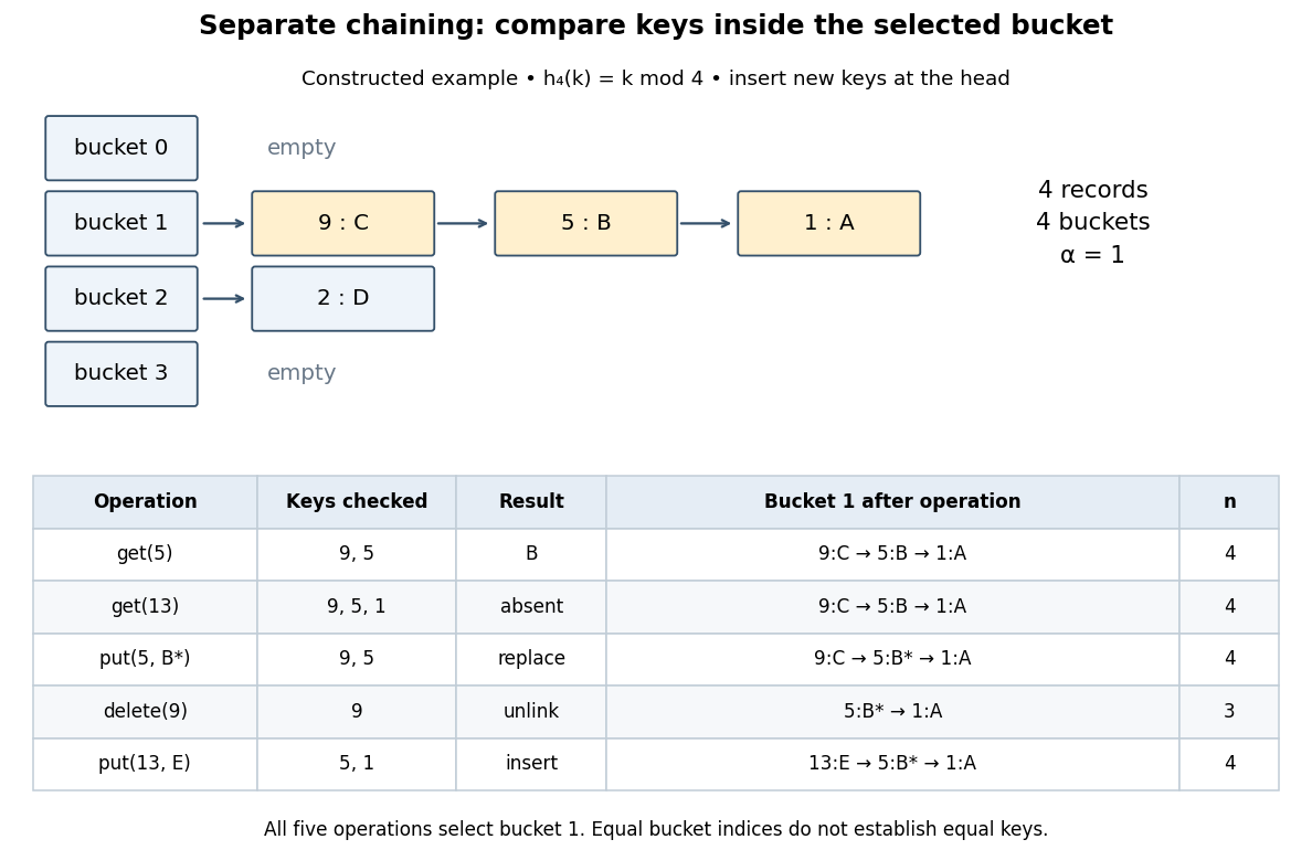
Separate chaining traces lookup, replacement, deletion and insertion through key equality
. Original deterministic model with . The table counts actual keys inspected, not elapsed machine time. Operations occur from top to bottom; only an absent key adds a new record, and the untouched record remains in hash bucket . Details.
get(5) rejects key , accepts key , and returns after two key equality comparisons. get(13) rejects and reports absence after three comparisons. put(5,B*) examines and replaces the value without changing . delete(9) examines just the head record, removes it, and gives . Finally, put(13,E) rejects before inserting the new head record; returns to and the chain is . The successive hash table load factors are . These counts follow from the stipulated chain order; a different insertion policy changes the successful-search counts.For a chain of length , lookup and deletion by key take time complexity in Big O notation. The same applies to
put before any resizing, since replacement semantics require checking for an existing equal key. Head insertion alone is if absence is already known; that is a different precondition. These bounds assume bucket-index hashing, array access, key equality comparisons, allocation and link updates. A long string or large integer can make hashing or comparison depend on its encoded length, so counting record visits alone does not establish constant running time.Under simple uniform hashing, each distinct key's bucket index is an independent random variable with a uniform distribution on a finite set of indices. The keys and query are fixed independently of this random assignment. Then lookup has expected time complexity, where is the hash table load factor; it is expected when stays bounded. These are model assumptions, not an automatic consequence of using a deterministic hash function.[ref]
Lecture 8: Hashing I. 6.006 Introduction to Algorithms, Fall 2011 by Massachusetts Institute of Technology, 6.006 course staff; pp. 4–5, chaining worst case and simple uniform hashing assumption
Here is the short calculation. For an absent query and stored keys , let be the indicator random variable of . The number of records inspected has expected valueby linearity of expectation. For a present fixed query, scanning its entire chain inspects at most itself plus all other colliding records, with expected value ; stopping at the match only decreases this upper bound. Adding constant hashing and bucket access yields expected for either query. The argument needs pairwise collision bounds; it does not require all the indicator random variables to be independent. A universal hash family can provide a related bound by random choice of a hash function for a fixed key set, as explained in that article.
The worst case remains , and an absent query takes comparisons if all records occupy its hash bucket. For instance, all collide under . Separate chaining remains correct, but a sequence of insertions that each checks the existing chain can take quadratic total work. Amortized analysis of resizing does not remove this search cost, and an adaptive choice of keys based on a known hash function is outside the stated simple uniform hashing model.
How soon should a hash collision appear? Specify the probability distribution of the outputs first. Evaluate distinct keys and assume their hash values are independent random variables, each with the uniform distribution on a finite set of possible outputs. The randomness may come from an idealized randomly chosen hash function; a fixed hash function and a fixed list of keys have a definite outcome. Sampling the same key twice creates a repeated hash value without creating a hash collision, so distinctness of the queried keys matters.
This is the existing birthday problem, with hash values in place of birthdays. Let be the probability of at least one equal pair. The exact formula isThe empty product is , so . Given previous distinct hash values, the next value avoids them with conditional probability . Multiply these conditional chances and subtract from . Equivalently, for , exactly of the equally likely ordered outcomes have no repeated value. This derivation also explains why independence of all outputs, rather than merely uniform individual values, is required.[ref]
https://cacr.uwaterloo.ca/hac/about/chap2.pdf. Menezes, van Oorschot and Vanstone, Handbook of Applied Cryptography, section 2.1.5, Fact 2.27(i), birthday probability
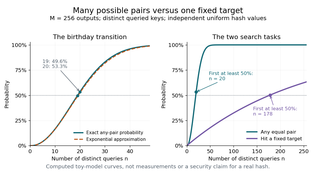

For , the exact hash collision probabilities are , , and . Thus only distinct queries already exceed a one-half chance of some pair matching. The striking feature is the number of opportunities: queries supply pairs. By linearity of expectation, the expected value of the number of equal pairs is . This expectation counts pairs, not the probability of at least one pair; three equal outputs contribute three pairs in one outcome. The union bound gives .
Using the natural logarithm expansion in the exact product givesFor , the omitted correction in the logarithm of the no-collision probability is . Thus the approximation is controlled when is small; in particular it becomes accurate at the birthday scale proportional to as increases. The inequality also shows that the displayed approximation is a lower bound for when . Setting its exponent to gives the approximate half-probability sample size for large .
For comparison, under the same independent uniform model the probability of hitting one previously fixed digest in queries isEach query supplies one chance to hit , instead of a growing number of possible pairs. For , , and the first integer with is . In a toy model with possible -bit digests, the any-pair transition therefore has scale queries, while the fixed-target transition has scale . This explains the birthday-search distinction between collision resistance and preimage resistance.[ref]
https://cacr.uwaterloo.ca/hac/about/chap9.pdf. Menezes, van Oorschot and Vanstone, Handbook of Applied Cryptography, Fact 9.33 and section 9.7.1, generic collision versus preimage searches
The assumptions are essential. Uniform marginals alone do not give the product formula: if all equal one shared uniform random variable, every distinct pair collides with probability . A universal hash family bounds each pair's hash collision probability, but that condition alone does not supply joint independence of every output. Nor does a fixed output length establish collision resistance or preimage resistance: the toy has , making deliberate hash collisions immediate. The curves describe the specified model and do not establish the security of a concrete cryptographic hash function.
If parental genotype frequencies are and the two parental gametes are independently sampled from the same allele pool, Mendelian segregation gives allele frequency . Their independent union has the displayed Hardy-Weinberg proportions, irrespective of parental genotype proportions. Equal allele frequencies in the two sexes and no transmission or viability distortion are part of this conclusion.
Multiplicative penetrance preserves Hardy-Weinberg equilibrium by  Codex 0 Created 2026-10-13 Updated 2026-11-05
For ordered alleles independently drawn with probabilities , suppose disease penetrance is . Conditional on disease, the allele draws remain independent with probabilities . This follows by normalizing the product . Unordered homozygote probabilities are and heterozygote probabilities are . Unaffected controls do not generally share this factorization: their genotype weights contain .
// Target: biology.bigb
Online text: people.math.ethz.ch/~acannas/Papers/handbook.pdf
Cited passages: Symplectic Geometry, §1.1, pp. 82–83: paired bases and Lagrangian spans; §1.5, pp. 90–91: Darboux coordinates; §1.1, p. 83: e-then-f basis and its block matrix; the coordinate formula follows by bilinearity.
There are unlisted articles, also show them or only show them.