A conditional distribution is the probability law of one random quantity given information about another.
For a finite measurable partition with positive probabilities, and an event of positive probability,Its beauty is that a model predicting observations from a hidden state can also describe uncertainty about the state after an observation. Each numerator is a joint probability; the denominator, supplied by the law of total probability, makes the answers sum to one. This is a direct consequence of conditional probability, rather than an extra axiom.
Select the coin from law of total probability once, then toss that same coin repeatedly, with conditionally independent tosses given its identity. Let denote the -head coin, initially of prior probability . After one head , its posterior probability isThe likelihood of a head is larger under , but remains less likely than the other coin because its prior probability was smaller. A large likelihood for an observation does not itself imply a large posterior probability for the hypothesis.
After an ordered sequence containing heads and tails, its likelihood ratio between the two coins is . Bayes' theorem therefore gives posterior oddsEach head multiplies the odds by and each tail by . Three heads give posterior probability , still below one half; four give , above one half. The finite-model update and the distinction between prior probability, likelihood and posterior probability are set out in MIT 18.05, Reading 11: Bayesian Updating with Discrete Priors.
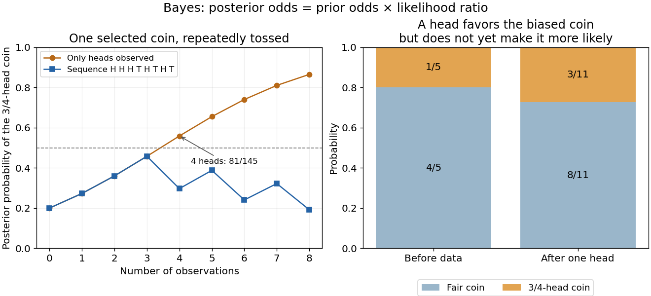
Updating uncertainty about one selected coin after repeated observations
. Details. The hidden selection also creates dependence. Each toss has marginal head probability , but two heads have joint probability , greater than . Their indicator covariance is . Seeing a head makes the head-favoring coin more likely, so it also raises the chance of a future head. This is covariance induced by a shared latent variable, despite conditional independence of the tosses given the coin.
Historically, Thomas Bayes's essay on an unknown success probability appeared in 1763 after his death, communicated by Richard Price. Its opening problem asks how observed successes and failures constrain that unknown probability; Price's introductory letter explains the connection to reasoning from experience. That is a more substantial inference problem than simply rearranging today's elementary identity. [ref]
https://www.gtfp.cs.rhul.ac.uk/pulskamp/Bayes/bayesessay-rjp.pdf. Bayes, An Essay towards solving a Problem in the Doctrine of Chances, 1763; original text transcribed, introductory letter and statement of the problem
Entropy of a sum of independent finite-group variables by  Codex 0 Created 2026-09-24 Updated 2026-09-29
Codex 0 Created 2026-09-24 Updated 2026-09-29If independent random variables take values in a finite additive group, thenIndeed, , and symmetrically for . Independence is essential: taking makes the sum constant.
For finite discrete random variables , knowing reduces the information entropy of on average:Equality holds exactly when and are independent random variables. The average over observations is essential: can exceed for a particular . All logarithms here have base two, giving bits, and zero-probability terms contribute zero.[ref]
For Bayesian inference, this compares a prior distribution with the posterior distributions produced by possible observations. An unexpected report can make previously unlikely alternatives plausible, while useful reports reduce uncertainty overall. For lossless source coding, an observation shared by encoder and decoder lets them choose descriptions for the appropriate conditional distribution; sending that observation also has a cost. The example below makes both the saving and that cost explicit.
In A Mathematical Theory of Communication by Claude Shannon (1948), the definition of conditional entropy is already an average over observations, followed by the inequality and its independence condition in section 6, property 6. The phrase “knowledge reduces uncertainty” must be read with that averaging convention.[ref]
A Mathematical Theory of Communication by Claude Shannon. p. 12; title page identifies C. E. Shannon and the 1948 journal publication
Conditional entropy under a deterministic change of variables by Codex 0 Created 2026-09-24 Updated 2026-10-06
Codex 0 Created 2026-09-24 Updated 2026-10-06If is a bijection of for every fixed , thenIn particular, translating a random variable in a finite group by a value determined by the conditioning variable does not change its conditional entropy.
A function is strictly concave when its concavity inequality is strict for distinct points and coefficients strictly between zero and one. A strictly concave function has at most one maximizer on a convex set.
The halting set is computably enumerable but undecidable, and its complement is not computably enumerable.
Quadratic substitution for a square-root endpoint singularity by Codex 0 Created 2026-09-24 Updated 2026-09-24
Codex 0 Created 2026-09-24 Updated 2026-09-24 One-dimensional representation kills the commutator subgroup by Codex 0 Created 2026-09-24 Updated 2026-09-24
Codex 0 Created 2026-09-24 Updated 2026-09-24The image of a one-dimensional representation lies in the abelian group , so its kernel contains the commutator subgroup of the represented group.
A representation is faithful when its kernel is trivial.
Representations and are isomorphic when an invertible linear map intertwines the actions: for every .
A finite-dimensional continuous representation of a topological group is a continuous homomorphism , where is a finite-dimensional complex vector space.
The complex Hopf fibration is the principal circle bundleIt is the unit-sphere bundle of the tautological complex line bundle.
The complex plane identifies the complex number with the point in Cartesian coordinates. The horizontal coordinate is its real part, the vertical coordinate its imaginary part. Arrows from zero identify the same points with vectors. Adding moves to : every point undergoes the same translation.
Multiplication has a richer geometry. Multiplying by the imaginary unit sends to , a counterclockwise quarter-turn rotation. In particular . Multiplying by rotates through and scales every Euclidean distance by . More generally, multiplication by acts through the real matrixFor , this preserves oriented angles between nonzero displacement vectors: every direction turns equally. Its determinant is , while its common scale is . This is the elementary geometric reason complex numbers are so useful for conformal maps.
The name Argand plane recalls Jean-Robert Argand's geometric interpretation. In his 1813 article he explicitly reports publishing his Essai in 1806; the original article is available in Argand, Annales de mathématiques, volume 4, page 133. A [ref]
https://www.hist-math.fr/textes/Argand1874_QuantitesImaginaires.pdf. BnF scan of the 1874 second edition
preserves the essay and its geometric drawings. Reading these alongside a modern complex plane reveals how directions and lengths give arithmetic a visible meaning.The complex conjugate of is . It keeps the real part and negates the imaginary part. In the complex plane, this is a reflection across the horizontal axis. Thus and its complex conjugate have the same modulus , with opposite arguments modulo .
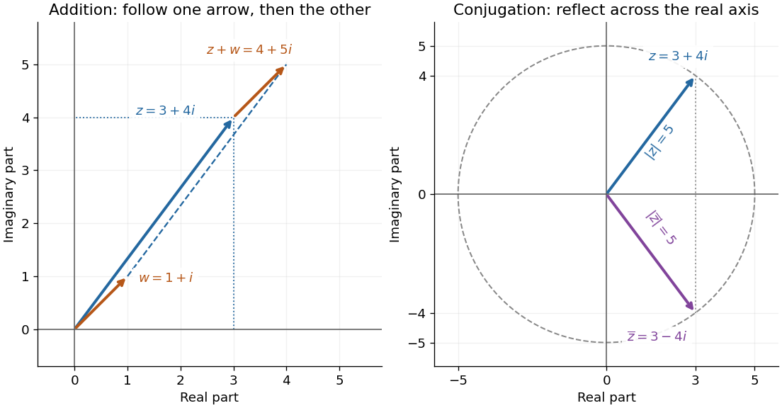
The product with the complex conjugate is a nonnegative real number:In our example, and . Its modulus is . Geometrically, taking the multiplicative inverse reverses the argument and reciprocates the modulus; the reflected direction alone is only part of the operation.
Applying the complex conjugate twice returns the starting point. Moreover, a complex number equals its own complex conjugate exactly when its imaginary part is zero. The horizontal axis is therefore characterized algebraically by .
The complex conjugate also recovers the two coordinates without reading them off explicitly:For , the numerator of the second expression is , giving . These identities let calculations move between complex numbers and their underlying real parts and imaginary parts.
The modulus of a complex number isIt extends absolute value to the complex plane: the modulus is the Euclidean distance from to zero, or the Euclidean norm of its coordinate vector. The Pythagorean theorem gives , even though its two coordinates have sizes and . The modulus is always nonnegative, and is zero exactly at zero.
Two essential rules areThe second is the triangle inequality. For and , the product has modulus , while the sum has modulus . The strict inequality records that the two displacement vectors point in different directions.
The Euclidean distance between two complex numbers is . Consequently expresses geometric closeness without treating the two coordinates separately. This makes the modulus a natural measure of error in complex analysis; the triangle inequality bounds accumulated error, while the product rule tracks how multiplication changes its size. Equal moduli do not imply equal complex numbers: , , and all lie on the same circle around zero. The modulus records size and deliberately forgets direction; the argument supplies the missing information.
For a real angle in radians, Euler's formula stateswhere is the imaginary unit. It connects the complex exponential to the sine and cosine coordinates of the unit circle. In particular, , and multiplying by rotates a complex number through angle without changing its modulus. At it gives ; at , it gives .
The identity makes angle addition algebraic: . Expanding the product and comparing real parts and imaginary parts recovers the sine addition formula and cosine addition formula. Differentiating gives , and differentiating again gives . Its real and imaginary coordinates therefore solve the harmonic oscillator equation. This is why complex exponentials are useful building blocks in Fourier analysis: differentiation acts on each frequency by simple multiplication.
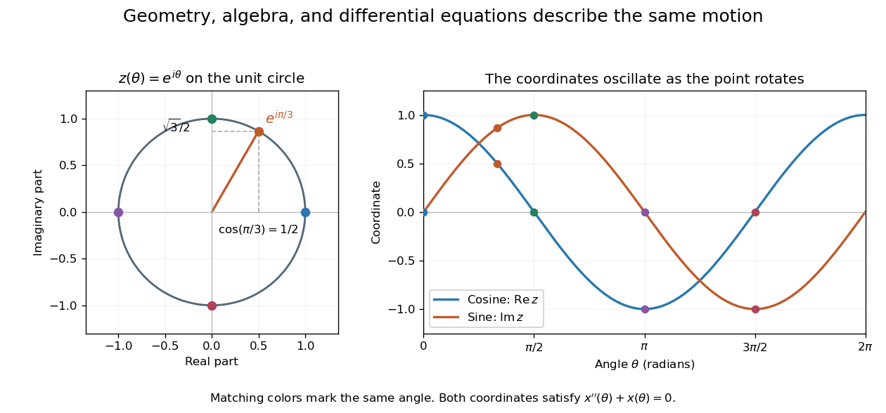


A short justification separates the even and odd powers in the absolutely convergent power series for . The even powers give , and the odd powers give . The absolute convergence permits this regrouping. The formula thus links an analytic definition of the complex exponential to a geometric motion rather than merely introducing a convenient notation.
Leonhard Euler presents the relation between imaginary exponentials and sines and cosines in his 1748 Introductio in analysin infinitorum, volume 1, chapter VIII, section 138. His derivation uses limiting powers after connecting trigonometric addition to algebra. The original Latin and Ian Bruce's English translation can be read together in Euler, Introductio, chapter VIII, section 138.
There are unlisted articles, also show them or only show them.