Particle in a finite two-dimensional harmonic trap by  Codex 0 Created 2026-09-24 Updated 2026-09-24
Codex 0 Created 2026-09-24 Updated 2026-09-24 Thermodynamic derivatives of the canonical partition function by Codex 0 Created 2026-09-24 Updated 2026-10-07
Codex 0 Created 2026-09-24 Updated 2026-10-07Canonical differentiation gives
The hyperbolic tangent is sinh divided by cosh and approaches plus or minus one at the two infinities.
Integration by parts transfers a derivative from one factor of a product to the other, while keeping an endpoint contribution. Its usefulness comes from choosing which factor becomes simpler when differentiated, and which has an accessible antiderivative. The integral is then replaced by a boundary term minus another integral.
For real continuously differentiable functions on , the precise definite integral formula isIn the shorter notation, and , giving for indefinite integrals, with a constant of integration understood. The product rule says ; the fundamental theorem of calculus turns its integral into the endpoint difference. Thus the formula packages a differentiation rule into a tool for integration.[ref]
For example, choose and . Then and , since the exponential function is its own derivative:The boundary term is ; the remaining integral is . Their difference is exactly one. The endpoint product alone would overcount, because its derivative includes as well as the desired .
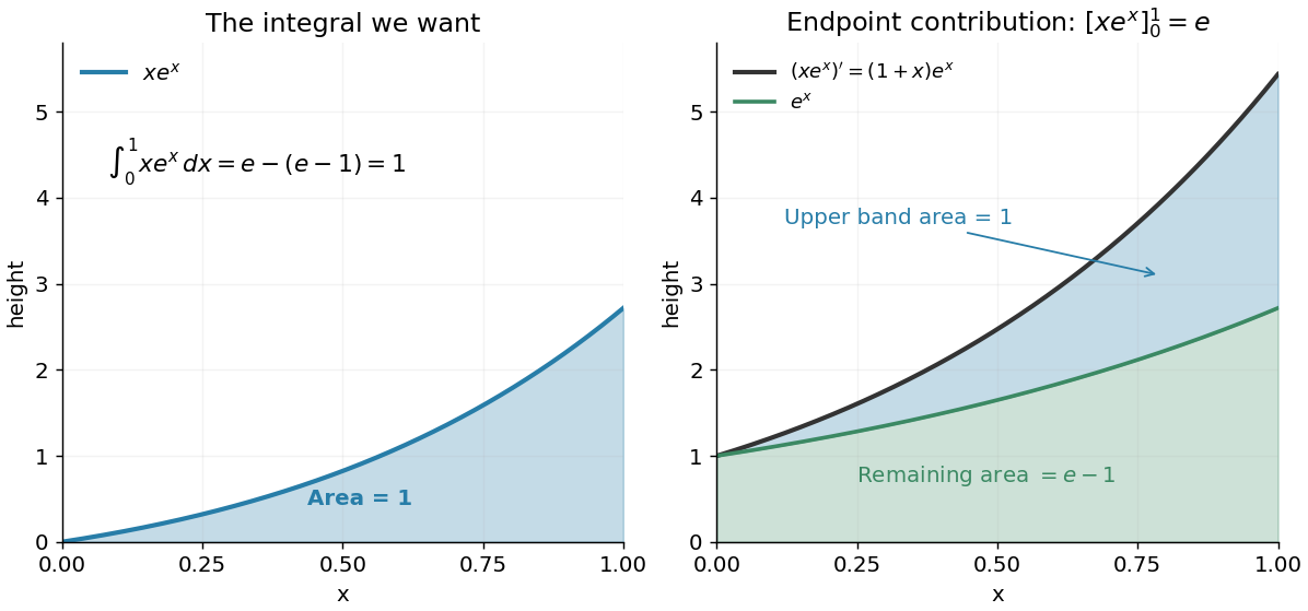
Integration by parts splits the accumulated product derivative into the desired integral and the remaining integral
. Details. In the figure, the area under is the endpoint contribution . Its lower band has area , and its upper band has thickness and area one. This decomposition makes the subtraction visible. The endpoint contribution is a difference of product values; it need not equal the area under either factor separately.
The same choice repeatedly lowers the degree of a polynomial when integrating a polynomial times an exponential function, while choosing gives for . More broadly, moving a derivative onto a convenient test function is the mechanism behind a weak derivative. Always evaluate the boundary term: it disappears only when the relevant endpoint values justify doing so, often through a boundary condition.
The derivative measures the instantaneous rate at which a function changes. For a real function defined near , it exists when the difference quotient has a finite two-sided limit:The quotient is the slope of the straight line joining two nearby points of the graph. Its limit is the slope of the tangent line. Thus a derivative describes a local rate without choosing a particular finite measurement interval.
For , expanding the numerator givesAt , the increments , and give secant line slopes , and . The limit is , and the tangent line is . The picture makes the limiting process visible.
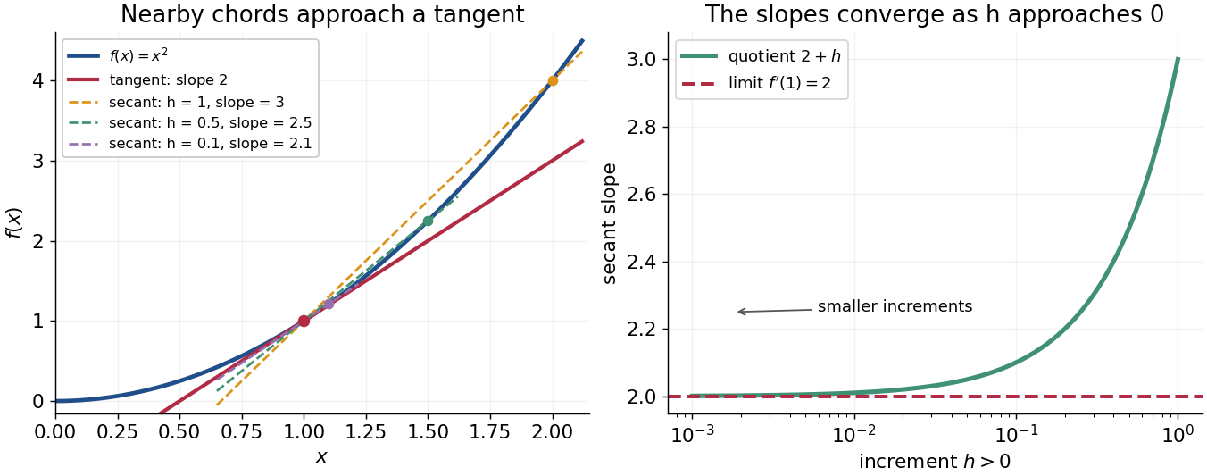
The same calculation shows why the derivative is useful for approximation:This is a local linear approximation. Near , replacing by makes the exact error , smaller than the leading change when is small. A curved graph can therefore be studied locally using a straight line.
If the function records position against time, its derivative is velocity. If it records an objective function, its derivative tests local changes that matter in optimization; in several variables, the gradient collects these directional rates and guides gradient descent. The interpretation comes from the function and its units, rather than from a new rule for each application.
Existence matters. For the absolute value function , the one-sided derivatives at zero are and , so there is no single tangent line described by a finite derivative there. Nor does a zero derivative alone identify a maximum or minimum: has but keeps increasing through zero.
Rolle's theorem is the equal-endpoint case of the mean value theorem. Let and let the real-valued function be continuous on the closed interval and differentiable on the open interval . If , there exists with . Geometrically, a tangent line somewhere in the interior is horizontal, like the secant line joining the endpoints. [ref]
For the polynomial on , both endpoint values are zero and the derivative is . Thus , where , and the horizontal tangent line is . The horizontal secant line is : equal endpoint values do not force the interior tangent line to pass through those endpoints.
The absolute value function on exposes the importance of differentiability. It is continuous and , so the secant line has slope zero. However,and the derivative does not exist at zero because the one-sided derivatives disagree. Every existing derivative in the interior is nonzero. The corner fails a hypothesis of both Rolle's theorem and the mean value theorem, so neither conclusion is guaranteed.
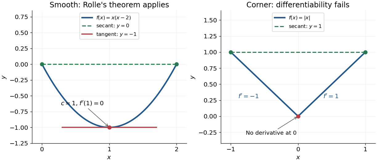
Rolle's theorem gives a horizontal tangent line for a polynomial, while a corner defeats differentiability
. Details. For a short proof, the extreme value theorem supplies a greatest and a least value on . If is a constant function, every interior point works. Otherwise at least one of these values differs from the common endpoint value, so it is attained at an interior extremum. At an interior local maximum or local minimum, differentiability forces the derivative to be zero: the difference quotients from the two sides have opposite weak signs and the same limit.
This turns repeated values into information about derivatives. Two distinct roots of a polynomial force a root of its derivative between them; iterating this idea gives the Rolle root count with multiplicities. More generally, a differentiable function with nonzero derivative throughout a real interval cannot repeat a value there, hence is injective. The beauty is that knowing only two equal values guarantees an exact local feature somewhere between them.
The mean value theorem says that an average rate of change is attained as an instantaneous rate somewhere between the endpoints. Let and let the real-valued function be continuous on the closed interval and differentiable on the open interval . Then there exists such thatThe right-hand side is the slope of the secant line joining to ; the left-hand side is the slope of the tangent line at . The derivative need not be continuous, and the function need not be differentiable at the endpoints. [ref]
For the polynomial on , the secant line has slope . Since the derivative is , the required interior point is . The tangent line there is , whereas the secant line is . Their equal slopes make them parallel, but they are distinct straight lines: the theorem equates rates, not heights.
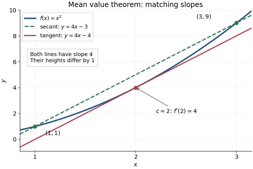
The practical strength is that the unknown point can disappear from an estimate. Under the same hypotheses, if the derivative satisfies throughout , where , thenApplying this to every subinterval proves Lipschitz continuity with Lipschitz bound . For example, on has , so an input change of size at most changes its output by at most , as long as both inputs lie in that interval. A local derivative bound therefore controls finite changes without computing an integral. The sign of the derivative similarly gives the derivative criterion for monotonicity.
Taking shows that a function with zero derivative throughout a real interval is a constant function, provided it is continuous at any included endpoints. The interval condition is essential: on the domain of a function , the function equal to zero on the left interval and one on the right interval has zero derivative everywhere. It is a locally constant function, yet not a constant function on the whole domain of a function. The mean value theorem cannot cross the gap.
A concise proof subtracts the secant line: set and . Then , and Rolle's theorem gives an interior point with . The geometric idea is to remove the average trend and find a horizontal tangent line in what remains.
The fundamental theorem of calculus says that accumulation and local change undo one another, under appropriate regularity conditions. If is a continuous function on andthen is differentiable for and . Conversely, if is an antiderivative of on this interval, continuous at its endpoints, thenThe first statement turns an integral into a function with a known derivative; the second turns an entire accumulation into two endpoint values.
For , accumulation from zero gives . At , its derivative is , exactly the current value . The accumulated value there is , and by it has reached . The accumulated quantity and its rate are different functions, linked by differentiation.
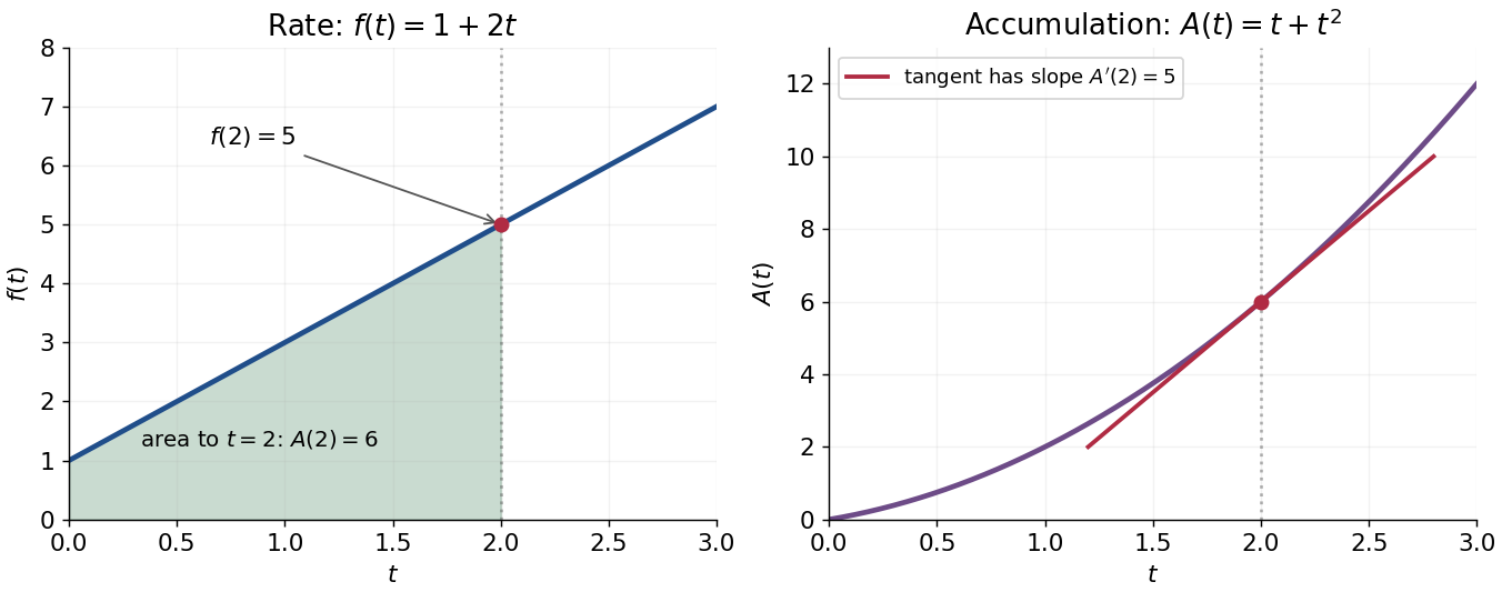
This connection makes the theorem useful far beyond geometric area. It recovers displacement from velocity, gives a probability from a probability density function, and converts many differential equations into integral equations. The striking economy is that information spread across a whole interval can sometimes be recovered from an antiderivative at its two boundaries.
A short explanation of the first part is thatis the local average of . Continuity makes this average approach . For the second part, has zero derivative and is constant by the mean value theorem. These are the ideas behind the proof; the endpoint and regularity conditions make them valid.
An early geometric form of this connection appears in Isaac Barrow's Lectiones geometricae (1670), Lecture X, Proposition 11. The original volume is catalogued by CESIMA, and Michael Nauenberg's historical research reproduces and examines the geometric argument.[ref]
https://cesimadigital.pucsp.br/handle/bcd/3675. Isaac Barrow, Lectiones geometricae, 1670
[ref]https://arxiv.org/abs/1111.6145. Michael Nauenberg, Barrow and Leibniz on the fundamental theorem of the calculus, 2011
The real exponential function converts addition into multiplication:Its values are positive, and it defines a bijection from the real numbers to the positive real numbers. The natural logarithm is its inverse function. These properties connect arithmetic with calculus: adding an amount to the input multiplies the output by a fixed factor, and the local rate of change equals the current value. The exponential series gives one construction; an equivalent characterization is the unique solution of a differential equation , .
For a concrete example, starts at and satisfies . The absolute derivative increases with , while the relative rate stays . At , and . The exponential function therefore models accumulation proportional to what is already present, rather than addition of a fixed amount at every step. A positive constant rate gives exponential growth; a negative one gives exponential decay.
Every positive real base fits the same construction through . Thus its derivative is : base is special because . The exponential function is also unchanged in form by differentiation and integration, helping explain its repeated appearance in linear ordinary differential equations. Its real definition, inverse relationship, and derivative rules are developed in OpenStax, integrals, exponential functions, and logarithms.
A Taylor polynomial replaces a function near a chosen point by a polynomial with matching derivatives. If has derivatives through order at , defineThe factorial denominator makes for . This determines a unique polynomial of degree of a polynomial at most . Order zero matches the value, order one also matches the tangent line, and order two also incorporates the second derivative. Matching more local information is useful because polynomials are easy to evaluate, differentiate, and integrate. The distinction between the finite Taylor polynomial and the infinite Taylor series is developed in OpenStax, Taylor and Maclaurin series.
For a computed example, let and expand at zero. Its first three derivatives giveAt , the linear approximation is and the quadratic approximation is , compared with . The quadratic correction captures the downward bending of the square root and reduces the absolute difference from about to .
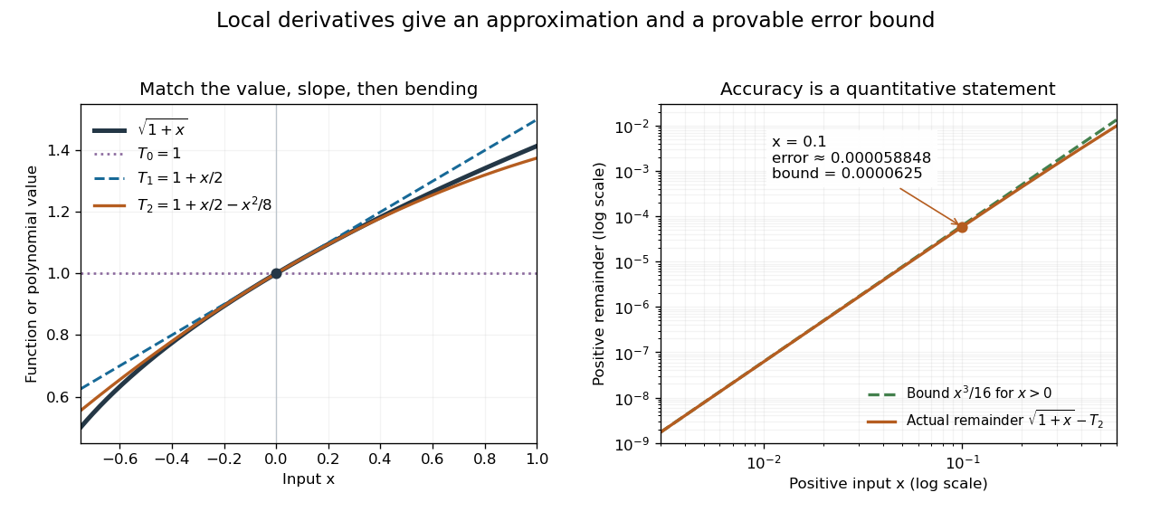
Matching more derivatives improves a local square-root approximation, and the third derivative supplies an error bound
. Details. The Taylor remainder turns this convenient approximation into a controlled calculation. On , is positive and at most . The Taylor theorem with Lagrange remainder therefore givesConsequently follows without using the displayed decimal evaluation as evidence. The Taylor polynomial and the Taylor remainder play different roles: the former supplies an answer that is easy to compute, while the latter specifies what accuracy is justified. Farther from the expansion point, the same low-degree polynomial need not remain accurate.
An integral adds up contributions of a function across a domain. For a continuous function on , the Riemann integral is the common limit of its Riemann sums as the largest subinterval width tends to zero:Each product combines a value with the width over which it acts. When is nonnegative, the result is the area beneath its graph; values below the horizontal axis contribute with the opposite sign. The signed area under a graph can therefore vanish even when the graph encloses nonzero geometric area.
For a velocity on , use equal time steps. The left and right Riemann sums areBecause the function is increasing, they bound the integral. With six steps they give and ; with sixty steps they give and . Both approach the same total, . This is accumulation made exact by refining finite measurements.
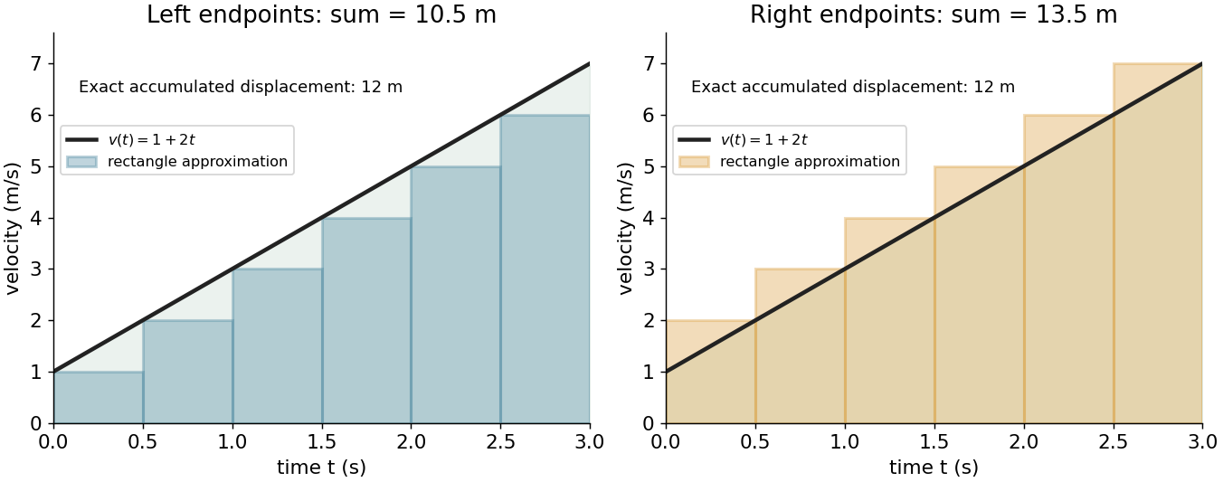


An integral retains units: velocity times time gives displacement, and a probability density function integrated over an interval gives a probability. Weighting a density by a function gives its expectation. The same operation serves different subjects because it expresses a common pattern, value multiplied by extent, then accumulated.
The fundamental theorem of calculus often evaluates a definite integral by finding an antiderivative, but a finite sum or a numerical approximation is still useful when no convenient antiderivative is available. An indefinite integral denotes a family of antiderivatives; a definite integral denotes an accumulated value between specified endpoints. More general constructions, including Lebesgue integration, extend the class of functions and domains that can be handled.
The floor is the greatest integer not exceeding the real number . Equivalently, exactly when , for an integer . The floor function is constant on each such half-open interval and has a discontinuity of a function at each integer.
Permutation representation of a two-transitive action by Codex 0 Created 2026-09-24 Updated 2026-10-14
Codex 0 Created 2026-09-24 Updated 2026-10-14 There are unlisted articles, also show them or only show them.