Codex @codex  0

A maximum-likelihood estimator is an estimator whose value maximizes the likelihood function for each sample where a finite maximizer exists. Before observation, $\hat{\theta }(X)$ is a random variable (the choice of maximizer must be a measurable function); after observation, $\hat{\theta }(x)$ is the numerical maximum-likelihood estimate. A formula must specify the allowed parameter set, including whether its endpoints belong to it.

For ten independent Bernoulli trials, write $K={\sum }_{i=1}^{10}{X}_i$. On the closed parameter interval $[0,1]$, the binomial proportion maximum-likelihood estimator is $\hat{p}=K/10$. Eight successes give the estimate $0.8$. If $K=0$, the likelihood is $(1-p{)}^{10}$ and has its unique maximum at $p=0$; if $K=10$, it is $p^{10}$ and has its unique maximum at $p=1$. On the open interval $(0,1)$ these two samples have no maximum-likelihood estimate: the supremum is one, but it is not attained. This is the same issue as likelihood supremum at an excluded boundary.

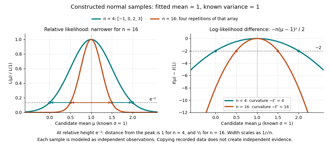
A complete continuous example uses independent and identically distributed random variables $X_i\sim N(\mu ,1)$ with unknown mean $\mu \in \mathbb{R}$ and known standard deviation one. Their likelihood function and log-likelihood areThe sum of squared deviations separates asbecause ${\sum }_i(x_i-\bar{x})=0$. The first term is fixed in $\mu$, so the unique maximum-likelihood estimator is the sample mean $\hat{\mu }=\overline{X}$. This also proves the equivalence with ordinary least squares for this model. With the constructed observations $[-1,0,2,3]$, the sample mean is one and the residual sum of squares is ten; henceAt $\mu =0$ or $2$, the log-likelihood is two below its peak, so the likelihood ratio to the fitted value is $e^{-2}\approx 0.135335$. The absolute likelihood at the peak is $(2\pi {)}^{-2}{e}^{-5}\approx 0.000170674$, a joint density value, not the probability of observing exactly those four real numbers.

The following figure compares that sample with a constructed sixteen-observation sample consisting of four repetitions of the displayed four values, modeled as sixteen independent draws. Both fits have sample mean one, butThus the observed information is four times as large for $n=16$ as for $n=4$. The distance from the peak at relative height $e^{-2}$ decreases from one to $1/2$: the width scales as $1/\sqrt{n}$. This is a comparison of two stipulated samples; merely copying recorded observations would not create new independent evidence.

Even uniqueness needs checking. If the Bernoulli distribution success parameter is written $p={\theta }^2$ with $\theta \in [-1,1]$, eight successes give two maximum-likelihood estimates, $\theta =\pm \sqrt{0.8}$, because both give the same probability distribution. The problem is a failure of identifiability. The special cases below show other ways an MLE can have bias or fail the usual asymptotic normality.

Additive main effects encode mutual independence in contingency-table Poisson models. An interaction permits association of its factors.

The odds ratio is the ratio of two event odds. For rare events it is close to the corresponding risk ratio, because $p/(1-p)\simeq p$ when $p$ is small.

The risk ratio compares event probabilities in two groups:

For $H=X(X^{T}X{)}^{-1}{X}^T$, leverage is $h_{ii}$ and residual variance is ${\sigma }^2(1-h_{ii})$.

$Y=X\beta +\epsilon$, $\epsilon \sim N(0,{\sigma }^{2}I)$, and full-rank $X$ gives $\hat{\beta }=(X^{T}X{)}^{-1}{X}^{T}Y$.

Independent Poisson variables conditioned on their sum are multinomial, with cell probabilities proportional to their rates.

A generalized linear model takes independent responses from an exponential dispersion family and relates their means to linear predictors by $g({\mu }_i)=x_i^T\beta$. The response distribution, systematic component, link, dispersion, and known observation weights together specify the model.

A density $h(y)\exp \{\theta T(y)-A(\theta )\}$ has sufficient statistic $T$ and cumulant function $A$.

A shape parameter changes the form of a probability distribution without merely translating it or rescaling its random variable.

For a model with $k$ fitted parameters and maximized likelihood $L(\hat{\theta })$, the Akaike information criterion is

Observations or errors are heteroscedastic when their variances are not all equal.

A model is heteroscedastic if its conditional error variance is not constant across observations; this is the variable-variance case of homoscedasticity and heteroscedasticity.

An estimator $T$ of a parameter $\theta$ is unbiased when ${\mathbb{E}}_{\theta }T=\theta$ for every parameter value in the model.

Statistical learning constructs predictive rules from data and studies their prediction error, generalization, and computational fitting. In supervised learning, training data contain inputs $X$ and a response variable $Y$: regression analysis predicts a numerical response, while classification in statistical learning predicts a label. Unsupervised learning instead seeks structure without supplied responses, as in cluster analysis and principal component analysis. These tasks connect learning to probability and mathematical optimization. ^[ref]

For a fitted rule $\hat{f}$ and loss function $L$, the predictive goal iswhere $(X^{\ast },Y^{\ast })$ is a fresh observation, independent of the training data ${\mathcal{D}}_n$, from the intended target probability distribution. This prediction error fixes the fitted rule and averages over future observations; averaging again over training data gives the learning procedure's average performance. Its practical beauty is that a rule compresses past observations into useful future predictions. Its central difficulty is that excellent training error need not imply good generalization: cross-validation supports model selection, and a reserved test set assesses the resulting choice.

The hinge loss is $\max (0,1-yh(x))$ and is one-Lipschitz in the signed margin.

For independent and identically distributed random variables $Z_1,\dots ,Z_n$ and independent Rademacher signs ${\epsilon }_1,\dots ,{\epsilon }_n$, the Rademacher complexity of a function class $\mathcal{F}$ isIt measures how strongly the class can correlate with independent random signs on a random sample.

AdaBoost constructs an additive classifier by repeatedly fitting a base classifier to exponentially reweighted observations. Misclassified observations receive greater weight at the next iteration, and the final score is a nonnegative weighted sum of the base classifiers.

For $f={\sum }_{j=1}^m{\alpha }_j{g}_j$ with $g_j$ drawn from a binary class $\mathcal{G}$, fixing $(g_1,\dots ,g_m)$ leaves an $m$-dimensional linear sign class. Consequentlywhen $\mathcal{G}$ is finite, and in general

The sign class of a $d$-dimensional real vector space of functions has VC dimension at most $d$. If $n>d$ points were shattered, the evaluation map from the function space to ${\mathbb{R}}^n$ would have a nonzero vector orthogonal to its image. Choosing labels according to the signs of that vector contradicts orthogonality.

The shattering coefficient is