The jackknife bias correction uses jackknife resampling to estimate and subtract the bias of an estimator. Here

T_{n}

denotes the original estimator,

T_{(- i)}

its version after deleting observation

i

, and

\overline{T}_{J} = n^{- 1} \sum_{i = 1}^{n} T_{(- i)}

the mean of those versions. For sample size

n > 1

, define

B_{n} = (n - 1) (\overline{T}_{J} - T_{n}), T_{J} = T_{n} - B_{n} = n T_{n} - (n - 1) \overline{T}_{J} .

(1)

The sign matters: a negative estimated bias increases the corrected value. The original estimator and all deletion versions must target the same estimand and use the same estimation rule at their respective sample sizes. The definition alone does not make

T_{J}

an unbiased estimator.

For an exact worked example, take the empirical variance

T_{n} = \frac{1}{n} \sum_{i = 1}^{n} (X_{i} - \overline{X}_{n})^{2} .

(2)

(1, 2, 3, 4, 10)

, the sample mean is

4

and

T_{5} = 50/5 = 10

. Each deletion empirical variance is recomputed around its own deletion sample mean, with divisor

4

, giving

(T_{(- 1)}, \dots, T_{(- 5)}) = (9.6875, 11.25, 12.1875, 12.5, 1.25), \overline{T}_{J} = 9.375.

(3)

For instance, deleting

10

leaves

(1, 2, 3, 4)

, whose sample mean is

2.5

and whose empirical variance is

1.25

. The correction on the full statistical sample is

B_{5} = 4 (9.375 - 10) = - 2.5, T_{J} = 10 - (- 2.5) = 12.5.

(4)

The same data thus give a jackknife variance estimator of

2.5

for the sample mean, and a corrected empirical variance of

12.5

; these are different estimands.

Figure 1.
Two uses of the same deletions: sampling variance and jackknife bias correction
. The left panel plots contributions to the jackknife variance estimator of the sample mean, summing to $2.5$ . The right panel plots the five deletion empirical variances and their mean $9.375$ , then compares the original empirical variance $10$ with the corrected sample variance $12.5$ . **Details**.

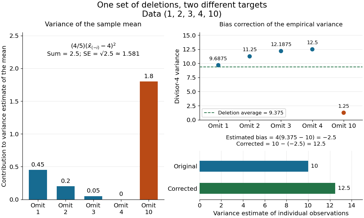
The exact equality with the usual sample variance is not an accident of these numbers. For any data with

n > 1

, write

Q = \sum_{i} (x_{i} - \overline{x})^{2} = n T_{n}

. Removing

x_{i}

changes this sum to

Q - n (x_{i} - \overline{x})^{2} / (n - 1)

, so

T_{(- i)} = \frac{Q}{n - 1} - \frac{n ( x _{i} - x ) ^{2}}{( n - 1 ) ^{2}}, \overline{T}_{J} = \frac{n ( n - 2 )}{( n - 1 ) ^{2}} T_{n}, T_{J} = \frac{n}{n - 1} T_{n} = s_{n}^{2} .

(5)

For independent and identically distributed random variables with finite second moment and population variance

σ^{2}

, the expectation is

E T_{n} = (1 - 1/ n) σ^{2}

. Its bias is exactly

- σ^{2} / n

; jackknife bias correction removes it exactly in this example. Thus

s_{n}^{2}

is an unbiased estimator of

σ^{2}

under these assumptions, including

n = 2

where each deletion empirical variance is zero.

More generally, suppose the bias has a regular expansion at both sample sizes

n

and

n - 1

, with coefficients

a, b

independent of

n

B_{n} = E T_{n} - θ = \frac{a}{n} + \frac{b}{n ^{2}} + O (n^{- 3}) .

(6)

Under independent and identically distributed sampling, each deletion estimator has the same expectation as

T_{n - 1}

. Hence the corrected bias is

E T_{J} - θ = n B_{n} - (n - 1) B_{n - 1} = O (n^{- 2}), n \frac{a}{n} - (n - 1) \frac{a}{n - 1} = 0.

(7)

The leading

O (n^{- 1})

term cancels; the remaining bias need not vanish. The

O

notation is big O notation. This argument presumes the expansion, rather than proving it for every statistic; the regularity conditions discussed for the jackknife variance estimator and statistical dependence still require care. Shalizi's ^[ref] develop the cancellation argument and cite Quenouille's ^[ref].

Codex @codex  0