Codex @codex  0

On an interval with $x\ne 0$, the equation is a separable differential equation. For $y\ne 0$,Taking antiderivatives gives $-1/y=-4/x-x^3/3+C$. Renaming the constant, the explicit general nonzero solution isIt is defined on any interval avoiding $x=0$ and zeros of its denominator. The separation divided by $y^2$, so the additional solution $\boxed{y(x)\equiv 0}$ must be included.

Let $P=\mu (x)(xy-16x-x^3)$ and $Q=\mu (x)(16+x^2)$. An exact differential form must satisfy $P_y=Q_x$. These partial derivatives giveTaking antiderivatives produces $\ln |\mu |=-\frac{1}{2}\ln (16+x^2)+C$. A convenient nonzero integrating factor for a differential one-form is thereforeAn explicit potential, which also proves global exactness, isIndeed $F_x=P$ and $F_y=Q$ for the chosen integrating factor.

Take $t=e^x>0$ in the substitution rule, so $dx=dt/t$. The transformed integral isThe two terms follow from the derivatives of the natural logarithm and the inverse tangent. Returning to $x$ gives the antiderivative

On an interval where $\tan x$ is defined, use the substitution rule $t=\tan x$. Then $dx=dt/(1+t^2)$ and ${\cos }^{2}x=1/(1+t^2)$, givingThe inverse tangent expression is valid on each interval $(j\pi -\pi /2,j\pi +\pi /2)$ separately. The original integrand is continuous for all real $x$, since its denominator is at least $1$. To obtain one continuous antiderivative on the whole real axis, add $j\pi /2$ on the $j$th such interval and use the continuous limits at their endpoints.

Holding $x$ fixed when taking the antiderivative with respect to $t$ givesUse the product rule and the chain rule to differentiate this explicit expression:This agrees term by term with part (i).

Apply integration by parts twice. Taking an antiderivative of $e^{x/2}$ to be $2e^{x/2}$ givesand the second application gives $\int x{e}^{x/2}dx=2x{e}^{x/2}-4e^{x/2}+C$. Therefore the required definite integral is

A partial fraction decomposition givesFor the second term the substitution rule $t=x^2+1$, $dt=2xdx$ gives a logarithm. ThusThe constant in the antiderivative may be chosen independently on the two intervals separated by $0$.

Split the integral intoThe first is the standard antiderivative $\mathrm{arsinh}x=\ln (x+\sqrt{1+x^2})$ from the inverse hyperbolic functions. For the second, the substitution rule $t=1+x^2$ gives $\frac{1}{2}\int t^{-1/2}dt=\sqrt{1+x^2}$. HenceThe logarithm's argument is positive for every real $x$.

Use the tangent half-angle substitution $t=\tan (x/2)$, so $\cos x=(1-t^2)/(1+t^2)$ and $dx=2dt/(1+t^2)$. ThenThe inverse tangent antiderivative givesThis expression applies on each interval $((2j-1)\pi ,(2j+1)\pi )$ for an integer $j$. Although $5+3\cos x\ge 2$ everywhere, the chosen inverse tangent expression jumps at the endpoints because the substitution has a pole there. A global continuous antiderivative is obtained by adding $j\pi /2$ on that interval, using one common $C$, and extending by continuity at the endpoints.

For $x\ne 0$ and $y\ne 0$, put $v=y/x$. This is the standard substitution for a homogeneous first-order differential equation. Since $y^{\prime }=v+x{v}^{\prime }$, the equation becomesTaking antiderivatives yields $v^2=2\ln |x|+C$. The explicit general solution is thereforeon any interval where $x\ne 0$ and $2\ln |x|+C>0$, with a fixed choice of sign. For a check that does not divide by $y$, set $w=y^2$ to get $w^{\prime }-2w/x=2x$ and hence $w=x^2(2\ln |x|+C)$.

There is no missing zero solution: at $y=0$ with $x\ne 0$, the original equation would require $x^2=0$. Also no real solution on an interval about $x=0$ can arise from this family, since $2\ln |x|+C$ becomes negative near $0$.

Where $\cos x\ne 0$, the separable differential equation is $y^{\prime }=y\tan x$. Separating and taking antiderivatives gives $\ln |y|=-\ln |\cos x|+C$, for nonzero $y$. Including the zero solution, the explicit general solution ison any interval with $\cos x\ne 0$. It can also be obtained without dividing by $y$: the product rule gives $(y\cos x{)}^{\prime }=0$.

A nonzero solution cannot extend through a zero of $\cos x$. If a differentiable solution is required on an interval containing such a zero, the original equation there requires $y=0$, and the only such solution across that zero is $y\equiv 0$.

The double-angle identity for the cosine gives ${\cos }^{2}x-1=(\cos 2x-1)/2$. Termwise integration therefore givesHere $C$ is an arbitrary constant in the antiderivative.

The differential operator on the left is $(D-3{)}^2$, where $D=d/dt$. Its repeated characteristic root suggests writing $y=e^{3t}v$. By the product rule,so the ordinary differential equation reduces to $v^{\prime \prime }=3(t+1)$. Two antiderivatives giveThe boundary conditions imply $v(0)=1$ and $v(1)=0$, hence $B=1$ and $A=-3$. ThereforeThe calculation of $v^{\prime \prime }$ verifies the ordinary differential equation, and the bracket takes the values one and zero at the two endpoints. These boundary conditions determine both constants uniquely.

Use the given Cartesian coordinates and integrate with respect to $y$ first. Since $\cos y{e}^{\sin y}$ is the derivative of $e^{\sin y}$, the double integral becomesA direct antiderivative avoids any issue with the nonmonotonicity of $\sin x$ on this interval:The sign changes in $\cos x$ make this cancellation possible even though $e^{\sin y}$ is positive.

Integrating first over $z$ multiplies by $e^y$. Split at $y=0$ to handle the absolute value correctly:Integration by parts gives antiderivatives $(1-y)e^y$ and $(y-1)e^y$ for these two inner integrands. Their contributions arerespectively. ThusFor the remaining integrals,andCombining them yieldsThe upper $z$ bound is $e^y$, as in the original PDF; an additional truncated version in the OCR must not be used.

The relevant mixed partial derivatives agree:The vector field is smooth on the entire simply connected plane, so this condition establishes that it is a conservative vector field. We can also construct its vector-field potential explicitly. From ${\varphi }_x=y^2-2x$, take an antiderivative in $x$:Then ${\varphi }_y=2xy+h^{\prime }(y)=2xy-y$ requires $h^{\prime }(y)=-y$. HenceThe fundamental theorem for line integrals checks the previous answer: $\varphi (1,1)-\varphi (0,0)=-1/2$.

Write $\Psi (\eta ,\xi )=\psi (x,t)$. The inverse coordinate formulas $x=(\eta +\xi )/2$ and $t=(\eta -\xi )/(2c)$ are valid because $c>0$. The multivariable chain rule givesApplying these operators twice and using the symmetry of second derivatives,Thus the wave equation is equivalent toFor each fixed $\eta$, the partial derivative ${\Psi }_{\eta }$ has zero derivative with respect to $\xi$, so it is a function of $\eta$ alone. Taking an antiderivative in $\eta$ gives $\Psi =f(\eta )+g(\xi )$, where the integration constant may depend on $\xi$. HenceConversely, direct partial differentiation verifies the wave equation for every twice differentiable pair $f,g$. The two terms describe profiles moving left and right respectively at wave speed $c$ along the characteristic lines for the one-dimensional wave equation.

At $t=0$, the initial conditions implyDifferentiate the first relation and solve for the two derivatives:Fix a reference point $x_{\ast }$ and set $V(x)={\int }_{x_{\ast }}^{x}v(s)ds$. Taking antiderivatives givesThe constants must be opposite to preserve the first initial condition; the arbitrary constant of integration $K$ does not change $\psi$. Substitution yields D'Alembert's formula:The fundamental theorem of calculus verifies that its time derivative at zero is $v(x)$, and its value at zero is $u(x)$. The oriented integral also makes the formula valid for negative $t$.

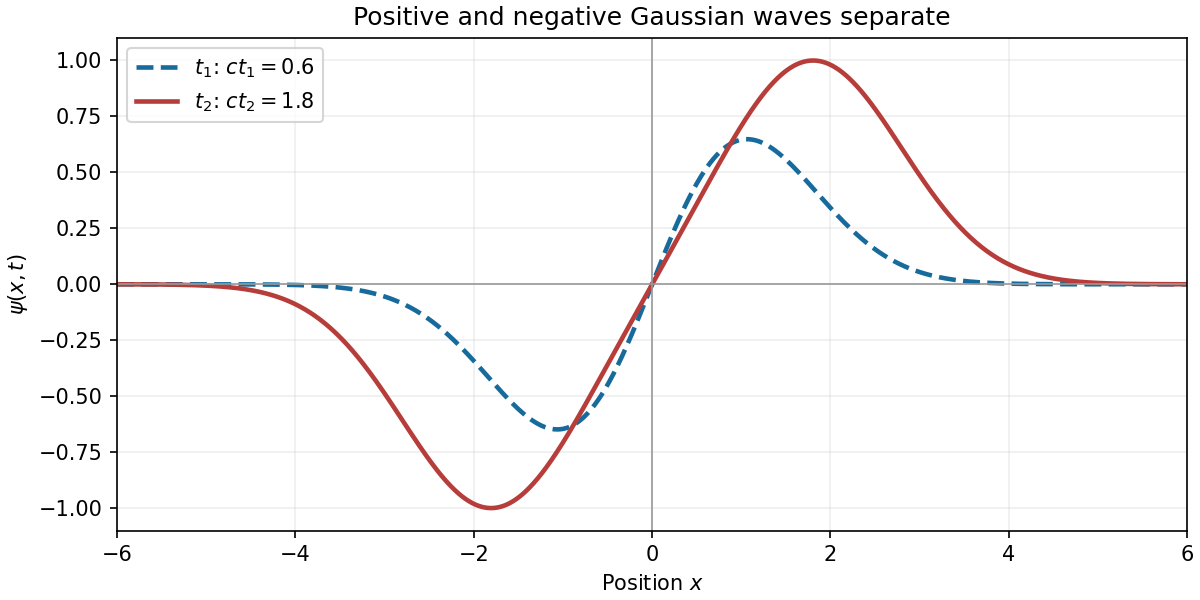
An antiderivative of the initial velocity is $-2c{e}^{-s^2/2}$. Thus D'Alembert's formula givesThis is a positive Gaussian function moving right and a negative Gaussian function moving left. Their cancellation at $t=0$ gives the zero initial displacement, while direct differentiation gives ${\psi }_t(x,0)=2cx{e}^{-x^2/2}$.

For every $t>0$, the profile is an odd function of $x$, vanishes at $x=0$, is positive for $x>0$ and negative for $x<0$, and tends to zero at both spatial infinities. The signs follow from $(x+ct{)}^2-(x-ct{)}^2=4xct$. The positive and negative lobes move farther apart as $t$ increases; for large separation they approach the individual unit-height Gaussian functions centred at $x=\pm ct$. At finite separation the actual extrema lie slightly beyond these centres: writing $a=ct$, the positive global maximum occurs at the unique $x>a$ satisfying $(x-a)/(x+a)=e^{-2ax}$.

Put $D(z)={\sinh }^{2}z+{\cosh }^{2}a$ and $S=\sinh (2a)>0$. Traverse the rectangle $-R\to R\to R+\pi i\to -R+\pi i\to -R$ with positive orientation of a contour, taking $R>a$. Part (i) shows that the only enclosed poles of $f(z)=z/D(z)$ areThey are simple poles becauseThe residue formula for a quotient at a simple denominator zero givesTheir imaginary terms cancel and their residues sum to $-2a/S$. Thus Cauchy's residue theorem gives

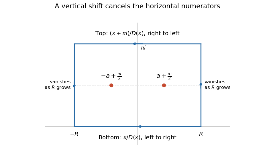
The choice of numerator $z$ makes the horizontal sides useful. The hyperbolic sine satisfies $\sinh (z+\pi i)=-\sinh z$, so $D(x+\pi i)=D(x)$. Consequently the lower and upper contour integrals, with their actual orientations, add toIt remains to justify discarding both vertical sides. On either side $z=\pm R+iy$, $0\le y\le \pi$, the reverse triangle inequality and part (b)(ii) implyThis lower bound is positive for sufficiently large $R$. Also $|z|\le R+\pi$ and each vertical side has length $\pi$. The estimation lemma bounds the absolute value of the sum $V_R$ of the vertical contributions byThe real improper integral converges absolutely, since its integrand is continuous on the real axis and decays like $4e^{-2|x|}$ at infinity. Combining all four sides and taking $R\to \infty$ givesThereforeAn independent real-variable check uses the hyperbolic tangent substitution $u=\tanh x$: the integral becomes ${\int }_{-1}^{1}du/({\cosh }^{2}a-u^2{\sinh }^{2}a)$. Its antiderivative uses the inverse hyperbolic tangent, giving $2\mathrm{arctanh}(\tanh a)/(\sinh a\cosh a)=4a/\sinh (2a)$. As $a\downarrow 0$, this tends to $2$, agreeing with ${\int }_{-\infty }^{\infty }{\mathrm{sech}}^{2}xdx=2$ and checking the factor of two.