Codex @codex  0

A Bayes factor measures how data change the relative support for two specified statistical models. Write $m_j(D)=p(D\mid H_j)$ for their Bayesian model evidence and define the direction explicitly:For positive finite $m_0(D),m_1(D)$, a value above one favors $H_1$ over $H_0$; a value below one favors $H_0$ over $H_1$. Reversing the comparison gives $B_{01}={\mathrm{BF}}_{01}=1/{\mathrm{BF}}_{10}$, the opposite direction used in some formulas below.

For mutually exclusive, exhaustive $H_0,H_1$ with positive prior probabilities, divide their two Bayes' theorem formulas. Their common data normalizer cancels, leavingThe Bayes factor therefore multiplies prior odds into posterior odds. It is evidence conditional on the specified statistical models and their within-model prior distributions; it is not $\mathbb{P}(H_1\mid D)$. Model prior probabilities supply a separate input.^[ref]

For an original stipulated example, consider ten independent and identically distributed Bernoulli trials, with heads as success. Compare $H_0:p=0.4$ with $H_1:p=0.7$, both fixed before seeing the data. Take $D$ to be one particular ordered sequence containing eight heads and two tails. The likelihood function under either point model is $p^8(1-p{)}^2$, soIf $\mathbb{P}(H_1)=0.1$, the prior odds for $H_1$ against $H_0$ are $1/9$. Hence the posterior odds are $21.9909706/9\approx 2.4434412$, andEqual model prior probabilities would instead give ${\mathrm{BF}}_{10}/(1+{\mathrm{BF}}_{10})\approx 0.956505$. The same Bayes factor can thus accompany different posterior probabilities. These statements condition on the two-model comparison; they do not establish that either statistical model describes a real coin.

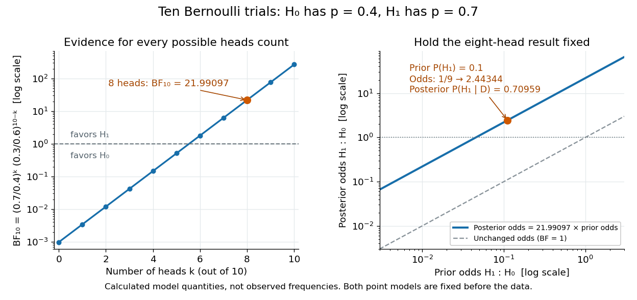
Using the heads count $K=8$ instead of the ordered sequence changes the sample space. The binomial distribution assigns it mass $\left(\genfrac{}{}{0ex}{}{10}{8}\right)p^8(1-p{)}^2$. The same binomial coefficient multiplies both models' Bayesian model evidence and cancels in their Bayes factor. Mixing an ordered-sequence numerator with a count denominator would introduce an erroneous factor of $45$.

Fix the candidate statistical models, their parameter prior distributions, and model prior probabilities before using the current data for this update. The Bayes factor is useful because it separates evidence from model prior odds, but it still depends on the parameter prior distributions. An improper prior has an arbitrary multiplicative normalization: multiplying its kernel by $c$ multiplies its formal marginal likelihood by $c$, even if the within-model posterior distribution is normalizable. Without a separately justified convention, the ordinary Bayes factor is then undefined up to arbitrary constants.^[ref]

The Bayesian model evidence is the prior predictive distribution evaluated at the data $D$. For a statistical model $H_j$ with a normalized prior density ${\pi }_j$, its marginal likelihood isThis is an expected value of the likelihood function under the prior distribution; for discrete statistical parameters, replace the integral by a sum. For continuous observations, $m_j(D)$ is a probability density function value with respect to a specified data reference measure, rather than a probability of one exact observation. Comparisons must use the same data and reference measure. The same $m_j(D)$ normalizes the within-model Bayesian posterior and supplies the between-model comparison in a Bayes factor.^[ref]

A normalized prior distribution makes the Bayesian model evidence an average, so it cannot exceed the largest likelihood function value on its support. A broad prior distribution can assign little mass to values that predict the data well, even when one value gives an excellent fit. The worked uniform-alternative binomial Bayes factor below makes the difference between averaging and maximum likelihood estimation explicit.

For Bayesian deviance $D(\theta )=-2\log L(\theta )$ under a common likelihood convention, define $\overline{D}=\mathbb{E}[D(\theta )\mid y]$ and $p_D=\overline{D}-D(\mathbb{E}[\theta \mid y])$. Then $\mathrm{DIC}=\overline{D}+p_D$ trades average fit against effective complexity. Lower values suggest better penalized predictive fit in comparable models; differences are not Bayes factors or model posterior probabilities. The choice of stochastic parameters and latent-variable representation matters, especially in a hierarchical Bayesian model.

A Gaussian practical-null mixture compares a narrow centered normal distribution prior with a wider centered normal distribution prior. Neither component is a point mass. With observed mean $y\mid \beta \sim N(\beta ,1/n)$ and prior precisions $q_0>q_1>0$, its model predictive variances are $V_i=1/n+1/q_i$, and the Bayes factor isThe overall posterior density is a Bayesian model averaging mixture with component means $ny/(n+q_i)$. A wide-prior penalty can favor the practical null near zero; its dominance depends quantitatively on both prior scales and the observation, not merely on the observation being of order $n^{-1/2}$.

For $n$ studies conditionally independent given the truth of one relationship, the event that at least one is positive has probability $1-{\beta }^n$ under the alternative and $1-(1-\alpha {)}^n$ under the null. Its Bayes factor therefore gives the displayed posterior odds. For interior error probabilities these tend back to the prior odds $R$. If power exceeds size, the Bayes factor decreases to one: the quotient of geometric sums is a weighted average of decreasing powers $[\beta /(1-\alpha ){]}^k$.

This result concerns the coarsened selection event. Full observed results instead multiply their individual Bayes factors, and concordant evidence can accumulate without this bound. It is a useful example of information discarded by publication bias.

For each observation time, use only the currently susceptible risk set $S_t$, with new-infection indicators $Y_{it}$. PutThis is the spatial Bernoulli infection model, under conditional independence of the indicators. Distances must be positive. Already infected trees should not be included as new susceptible trials. The minus sign in the power kernel is present in the original PDF, although it is absent in the converted TeX.

The parameter $\alpha$ must be nonnegative: for $\alpha <0$ and positive exposure, $1-e^{-\alpha A_{it}}<0$ is not a probability. Therefore the stated unrestricted normal prior distribution cannot literally define the model. A coherent interpretation is a normal prior distribution restricted to $\alpha >0$,Here $\Phi$ is the standard normal distribution function. Use the same proper prior distribution in both kernel models. The given Gaussian prior distributions for $\beta$ and $\gamma$ are mathematically valid on the real line for finite positive distances, though restricting them to positive values would impose decaying kernels and would require the corresponding normalized prior distributions.

The full conditional kernels areNeither is generally normal or another elementary conjugate family: the infection factors contain $1-e^{-\alpha A}$, and $A$ depends nonlinearly on $\beta$. Thus a simple conjugate Gibbs sampler is unavailable. This does not make Gibbs sampling logically impossible; exact rejection or slice conditional draws could be used if implemented. A straightforward alternative is Metropolis–Hastings algorithm updates within each coordinate.

For example, put $\eta =\log \alpha$ and use symmetric Gaussian random-walk proposals for $(\eta ,\beta )$. The target in these coordinates isThe factor $e^{\eta }$ is the Jacobian determinant and must be retained. Accept according to the ratio of this target, either for a block or one coordinate at a time. Posterior averages and quantiles of $e^{\eta }$ and $\beta$ estimate the requested marginal posterior distributions.

To compare kernels, introduce $M\in \{1,2\}$ with positive model prior distribution probabilities $w_1,w_2$. Under model two replace $A_{it}$ by ${\sum }_{j\in I_t}{e}^{-\gamma d_{ij}}$, defining $L_2(\alpha ,\gamma )$. The joint model/parameter target iswhere $\zeta =\beta$ or $\gamma$ and $p_M$ is its normalized proper prior distribution. Within each model use the preceding random-walk updates. For a concrete model switch, keep $\alpha$, propose the other model's kernel parameter independently from its prior distribution, and use equal forward and reverse switch-selection probabilities. A move from $(1,\alpha ,\beta )$ draws $\gamma \sim p_{\gamma }$ and has ratioAccept with the minimum of this ratio and one. The auxiliary-coordinate swap $(\alpha ,\beta ,\gamma )\mapsto (\alpha ,\gamma ,\beta )$ has absolute Jacobian determinant one, so no additional factor occurs; unequal switch-selection probabilities would require their reverse/forward ratio. This is a valid model-switching Markov chain Monte Carlo construction even though the two active models have equal parameter dimension. Prior distribution proposals may be inefficient, so fitted proposals can be substituted provided their probability densities remain in the acceptance ratio.

After checking mixing, estimate posterior model probabilities by the fractions of retained iterations in each model. The Bayes factor in favor of the first kernel isUse the posterior distributions within each model as well as these odds to assess the competing distance kernels. Proper prior distributions and their model-dependent normalizing constants are essential for this comparison.

For these two simple hypotheses the Bayes factor is the ratio of their normal probability densities:Therefore $\boxed{B_{10}(y)=e^{2.49(y-1.245)}}$, and the posterior odds are $R{B}_{10}(y)$.

Yes: replacing the observed statistic by a significance label loses information. The binary positive event has Bayes factor $(1-\beta )/\alpha \simeq 16$, but the observed-statistic Bayes factor varies continuously with $y$. A result just at the threshold has $B_{10}(1.65)\simeq 2.74$, while $B_{10}(3)\simeq 79.0$. Both would receive the same positive label.

The binary calculation is correct for that deliberately coarsened observation; its problem is treating it as the whole evidence when the statistic is available. This is the point developed in Goodman and Greenland's response.

Let $A_n$ denote the event that at least one study is positive. Conditional independence gives $\mathbb{P}(A_n\mid T)=1-{\beta }^n$ and $\mathbb{P}(A_n\mid F)=1-(1-\alpha {)}^n$. Updating the prior odds by this event's Bayes factor givesThese are the odds under at-least-one-positive selection, not the odds using every study's actual result.

For $0<\alpha ,\beta <1$, both event probabilities tend to one, so the posterior odds tend to $\boxed{R}$. If $1-\beta >\alpha$, the event's Bayes factor decreases toward one. To see monotonicity, put $a=1-\alpha >\beta$ and writeThe last quotient is a weighted average of the decreasing values $(\beta /a{)}^k$, with weights $a^k$. Adding the next, smaller value decreases the average.

Thus the selection rule becomes less informative as more teams try: eventually a positive study is almost certain even under the null. This explains the hotter-field interpretation in Ioannidis's model. It describes evidence retained by this particular selection event, rather than proving that every individual study becomes less reliable or that the full accumulated evidence gets weaker.

Consistent independent replications should strengthen confidence; contradictory results can weaken it. The change depends on the actual evidence. If $k$ of $n$ studies are positive and all labels are available, the posterior odds areFor the normal model, retaining the full independent statistics instead givesEach study multiplies the existing odds by its own Bayes factor. Reading a complete synthesis is therefore different from learning only that somebody obtained a positive result. Publication bias, dependence between studies and changes in study design must be accounted for before applying the independent-product formula.

A sufficient statistic $T$ has a conditional distribution of the data given $T$ that does not depend on the parameter. In a dominated family, the factorization criterion for sufficiency states that this is equivalent to $p_{\mu }(x)=h(x)g_{\mu }(T(x))$ for a nonnegative parameter-free $h$. Bayes' formula then gives a posterior distribution proportional to $\pi (\mu )g_{\mu }(T(x))$, because $h(x)$ cancels from numerator and normalizing denominator. Thus the posterior depends on the data only through $T$.

For the normal sample,The first term is parameter-free, so the factorization proves sufficiency of $\bar{X}$. Combining its likelihood with the normal prior and completing the square givesThe prior predictive distribution of the sample mean is obtained from $\bar{X}=M+\epsilon$, $\epsilon \sim N(0,1/n)$ independent of $M$:

Define the Bayes factor $B_{01}$ as the marginal likelihood under $H_0$ divided by that under $H_1$. The common residual factor cancels, so it is the ratio of the densities of $\bar{X}$ under these two hypotheses:The reverse Bayes factor is its reciprocal. At $|\bar{x}|=1.96/\sqrt{n}$,for a fixed positive $\tau$. Thus the frequentist test is at its rejection threshold while fixed prior odds give increasingly strong posterior support for the point null. This is the Jeffreys-Lindley paradox for a Gaussian point null: the standardized statistic stays fixed, but the observed effect tends to zero and the fixed-scale alternative spreads predictive mass much more widely. There is no logical contradiction, since the procedures compare hypotheses using different calibrations. For the degenerate $\tau =0$ the hypotheses coincide and $B_{01}=1$.