Codex @codex  0

Vector normalization converts a nonzero vector in a normed vector space into a unit vector. Absolute homogeneity of a norm givesThe direction is unchanged by multiplying by a positive real scalar. For $c>0$, $\Vert cv\Vert =c\Vert v\Vert$ and $\widehat{cv}=\hat{v}$; for a negative real scalar, $\widehat{cv}=-\hat{v}$. Thus $(3,4)$ and $(6,8)$ normalize to the same unit vector, while $(-3,-4)$ normalizes to its negative. This decomposition is useful for specifying a direction independently of a force, velocity or displacement magnitude.

In a complex normed vector space, a nonzero complex scalar $c$ instead gives $\widehat{cv}=(c/|c|)\hat{v}$. The remaining complex argument is not removed by normalization. For a pure quantum state, vectors differing only by this overall global phase represent the same physical state; vector normalization alone does not identify them.

The zero vector cannot be normalized this way. The construction also applies in a function space: an eigenfunction of a Sturm-Liouville problem can be scaled to unit weighted norm byThe positive weight $w$ specifies the weighted inner product. Multiplication by this nonzero constant preserves the eigenvalue equation and its homogeneous boundary conditions.

Use a velocity potential to reconstruct an irrotational flow from one scalar field. A velocity potential $\varphi (\mathbf{x},t)$ satisfiesIt has units ${\mathrm{m}}^2{\mathrm{s}}^{-1}$ and is unchanged as a description of the velocity field when any function of time alone is added. For twice continuously differentiable $\varphi$, the identity curl of a gradient proves zero vorticity. In incompressible flow, taking the divergence also gives ${\nabla }^2\varphi =0$, the Laplace equation. This turns a three-component velocity field into a single harmonic function with appropriate boundary conditions. ^[ref]

For uniform flow $\mathbf{u}=(U,0,0)$, take $\varphi =Ux$. With $U=2\mathrm{m}{\mathrm{s}}^{-1}$, the change from $x=0$ to $x=3\mathrm{m}$ is $\Delta \varphi =6{\mathrm{m}}^2{\mathrm{s}}^{-1}$. By the fundamental theorem for line integrals, the line integral of velocity between these points equals that change along any path in the domain; a closed curve gives zero circulation.

For the potential line vortex, choose a local angle branch in polar coordinates and set $\varphi =K\theta$. Then $u_r={\partial }_r\varphi =0$ and $u_{\theta }=r^{-1}{\partial }_{\theta }\varphi =K/r$. One counterclockwise turn changes the continued velocity potential by $2\pi K$, although the velocity field returns to its original value. With $K=1{\mathrm{m}}^2{\mathrm{s}}^{-1}$, this change is $2\pi {\mathrm{m}}^2{\mathrm{s}}^{-1}$, exactly the circulation. A full annulus therefore admits local angle branches and a multivalued velocity potential, but no global single-valued velocity potential when $K\ne 0$. Cutting the annulus along a radial line allows a single-valued angle branch on the remaining domain. The obstruction is path independence, not a failure of the local gradient formula.

Let $D$ be bounded, connected and simply connected, and let $u$ be a smooth divergence-free field. Suppose a sufficiently smooth vector field $A$ satisfies the displayed Poisson and boundary conditions. Divergence gives $\Delta \mathrm{div}A=0$ with zero boundary value, so harmonic uniqueness gives $\mathrm{div}A=0$. The vector Laplacian identity then implies $\nabla \times (\nabla \times A-u)=0$.

On a simply connected domain, define a scalar potential by integrating this curl-free difference along a path from a fixed point. Vanishing circulation around contractible loops proves path independence. Thus the difference is $\nabla \chi$; its divergence and boundary normal component give $\Delta \chi =0$ and ${\partial }_n\chi =0$. Green's identity yields ${\int }_D|\nabla \chi {|}^2=0$, proving the reconstruction. Additional conditions on $A$ can specify its own boundary problem; the argument assumes its existence and proves that its curl is exactly $u$. Simple connectivity is essential for eliminating possible non-gradient harmonic circulation fields.

The change in output voltage per input stress under specified geometry, loading direction, frequency and electrical boundary conditions.

The evolution of a vorticity distribution together with the velocity field it induces. A transport equation advances vorticity; diagnostic inversion recovers velocity from it and the specified boundary conditions.

The wave equation is a second-order linear partial differential equation describing waves with finite propagation speed. In one spatial dimension its homogeneous, constant-coefficient form isHere $x$ is position, $t$ is time, $u(x,t)$ is the disturbance, and subscripts denote partial derivatives. For a wave equation on a string, $u$ is transverse displacement; in linear acoustics, it can be a pressure perturbation. In several spatial dimensions, $u_{xx}$ becomes the Laplacian $\Delta u$. The same mathematical structure connects vibrating strings and acoustic waves, although their physical assumptions and wave speeds differ. ^[ref]

For the whole-line Cauchy problem, prescribe both displacement $u(x,0)=f(x)$ and velocity $u_t(x,0)=g(x)$. A classical solution has continuous partial derivatives through order two; $f\in C^2(\mathbb{R})$ and $g\in C^1(\mathbb{R})$ suffice for D'Alembert's formula to produce one. A finite string additionally needs boundary conditions. These statements concern the unforced model with constant $c$; damping, spatially varying coefficients and nonlinear terms change the solution formula.

A travelling wave $F(x-ct)$ carries its entire profile to the right at wave speed $c$; $G(x+ct)$ travels left. Their sum is again a solution by the superposition principle. A standing wave instead has a fixed mode shape whose size and sign oscillate: in $\sin (kx)\cos (ckt)$, each node of a standing wave stays stationary. The distinction is especially clear in the pulse and string diagrams below. For this ideal model, the dispersion relation is ${\omega }^2=c^2{k}^2$: each propagation branch is nondispersive, so a localized profile translates without spreading. This makes the equation a useful reference against which to understand wave dispersion and damping.

The appealing combination is local interaction with global predictability: neighbouring displacements determine acceleration through $u_{xx}$, yet D'Alembert's formula explicitly identifies exactly which initial locations can influence a later observation. Finite propagation speed turns that observation into a domain of dependence, rather than requiring knowledge of the entire initial string.

An ideal uniform, flexible string under constant tension $T>0$ has transverse displacement $y(x,t)$ satisfyingwhere $\mu >0$ is linear mass density, meaning mass per unit length of the straight reference string. The approximation assumes small slope $|y_x|\ll 1$, transverse motion, negligible bending stiffness, negligible damping, and no distributed external force. Constant tension and uniform linear mass density make $c$ constant. Some texts use $\rho$ for this same linear mass density, giving $c=\sqrt{T/\rho }$; here $\rho$ must have units $\mathrm{kg}{\mathrm{m}}^{-1}$, rather than units of volume mass density. ^[ref]

The units provide a useful check: $T/\mu$ has units $(\mathrm{kg}\mathrm{m}{\mathrm{s}}^{-2})/(\mathrm{kg}{\mathrm{m}}^{-1})={\mathrm{m}}^2{\mathrm{s}}^{-2}$. For $T=100\mathrm{N}$ and $\mu =0.010\mathrm{kg}{\mathrm{m}}^{-1}$, the wave speed is $100\mathrm{m}{\mathrm{s}}^{-1}$, so a pulse crosses a one-metre string in $0.010\mathrm{s}$. Quadrupling tension doubles wave speed; quadrupling linear mass density halves it. These square-root laws explain how material and loading set the time scale of the vibration.

For a length-$L$ string with fixed endpoints, the homogeneous Dirichlet boundary conditions are $y(0,t)=y(L,t)=0$. Its nonzero normal modes haveThus $cn\pi /L$ is an angular frequency, in radians per second, whereas $cn/(2L)$ is the frequency in hertz. The wavelength is $2L/n$, and each node of a standing wave lies at $x=jL/n$ for some $j=0,\dots ,n$. For the numerical string above with $L=1\mathrm{m}$, the first three frequencies are $50$, $100$ and $150\mathrm{Hz}$, with angular frequencies $100\pi$, $200\pi$ and $300\pi {\mathrm{s}}^{-1}$. ^[ref]

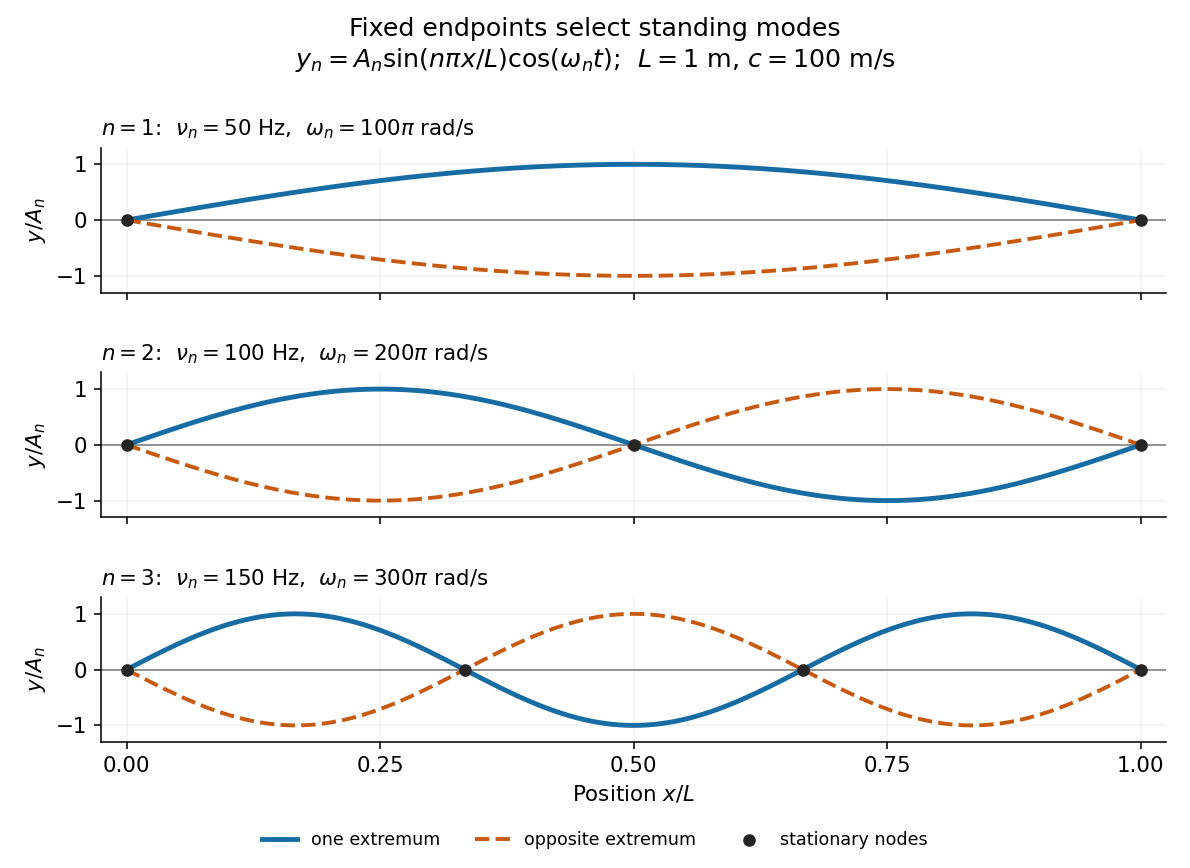
Each normal mode is a standing wave, but it also has a travelling wave description:At a fixed endpoint an incident displacement pulse reflects with reversed sign, allowing incident and reflected displacements to cancel at the endpoint. Periodic reflection for a fixed-end string implements both endpoints through odd, $2L$-periodic extensions of the initial data. This is the bridge between moving pulses and the stationary Fourier sine basis. ^[ref]

A short derivation comes from Newton's second law. The transverse force on a small segment is approximately $T[y_x(x+\delta x,t)-y_x(x,t)]$, and its mass is $\mu \delta x$. Dividing the force balance by $\delta x$ and taking the limit gives $\mu y_{tt}=T{y}_{xx}$. Separation of variables then gives ${\varphi }^{\prime \prime }+k^2\varphi =0$; the fixed-end boundary conditions select $k=n\pi /L$, while the temporal equation is a harmonic oscillator equation with $\omega =ck$.

A waveguide confines a wave transversely while allowing propagation along a longitudinal direction. Material properties and boundary conditions select transverse normal modes, whose longitudinal dispersion relations may have cutoffs even when the bulk material is nondispersive. Examples include an optical fiber, a hollow electromagnetic waveguide, and a membrane waveguide. Guiding reduces geometric spreading along the chosen route but does not eliminate absorption, scattering or leakage.

The wavelength $\lambda$ is the spatial period of a monochromatic wave, measured at a fixed time along the wavevector. For a plane wave with a sinusoid as its profile, it is the distance between consecutive wave crests, or between any consecutive points with the same wave phase modulo $2\pi$:Here $\mathbf{k}$ uses angular wavenumber, $f$ is ordinary frequency, and $v_p$ is phase speed. A distance between arbitrary zero crossings need not be a wavelength: consecutive zeros of a sinusoid are only $\lambda /2$ apart, with opposite slopes. In a standing wave, consecutive nodes of a standing wave are also $\lambda /2$ apart; $\lambda$ refers to the constituent travelling waves, even though the nodes of a standing wave do not travel.

Across a stationary interface between stationary linear media, the incident, reflected and transmitted monochromatic waves have the same frequency. The boundary conditions must hold at every time: terms oscillating with different angular frequencies cannot cancel throughout the entire time record. Each medium's dispersion relation then determines its own angular wavenumber and wavelength, soFor electromagnetic radiation in a transparent medium with refractive index $n$, $v_p=c_0/n$ and $\lambda ={\lambda }_0/n$, where $c_0$ is the vacuum speed of light. A synthetic example with ${\lambda }_0=600\mathrm{nm}$ and $n=1.5$ gives $\lambda =400\mathrm{nm}$ at the same frequency. This conservation argument assumes time-independent linear material response and a stationary interface in the chosen frame. A moving interface can produce a Doppler effect; time-dependent or nonlinear response can change or generate frequencies.^[ref]

A broad frequency spectrum generally supplies many component wavelengths, rather than one wavelength for an entire pulse. Even two tones have both their individual wavelengths and a different overall repetition distance: the $2$- and $8$-cycle-per-metre sum in spatial sampling of a wave repeats after $0.50\mathrm{m}$, but contains the finer $0.125\mathrm{m}$ structure. A narrow wave packet can have an approximate carrier wavelength; the wave envelope propagates approximately at group velocity, determined by the slope of the dispersion relation. Substituting that group velocity into $\lambda =v_p/f$ generally gives the wrong carrier wavelength. Where the medium varies slowly, local wavelength gives a more useful description.

A zero mode is a nonzero eigenvector of an operator with eigenvalue zero. For a differential fluctuation operator it must also satisfy the specified boundary conditions. A zero mode prevents ordinary inversion of the operator and makes its unmodified functional determinant vanish. Gauge directions can produce zero modes of a kinetic operator, while stationary-path focusing can produce them in a semiclassical boundary-value problem. Removing, separately integrating or otherwise treating these directions is necessary before using a Gaussian determinant formula.