Codex @codex  0

With interface normal from medium 1 to medium 2, Ampère's boundary condition is $\hat{\mathbf{n}}\times ({\mathbf{H}}_2-{\mathbf{H}}_1)={\mathbf{K}}_f$. With no free surface current, tangential $H$ is continuous. Normal $B$ is continuous independently because magnetic monopoles are absent.

For a negative Coulomb energy, remove the exponential decay and regular radial power to obtain a confluent-hypergeometric series. Its recurrence terminates only when $n=q+\ell +1$, with $q$ a nonnegative integer. Regularity at the origin and normalizability at infinity then give the hydrogenic energy levels. Without those physical boundary conditions the radial differential equation has other solutions.

Thermal conduction transfers heat through microscopic interactions without bulk transport of matter. To predict the heating load through a bar, combine Fourier's law with conservation of energy and the imposed end temperatures. In the isotropic model with positive thermal conductivity $k$, the conductive heat flux points from high to low temperature, opposite to the temperature gradient. A spoon warming along its handle and heat escaping through a wall are familiar examples.

Consider a bar of length $L=0.10\mathrm{m}$, constant cross-sectional area $A=0.010{\mathrm{m}}^2$ and constant thermal conductivity $k=2\mathrm{W}{\mathrm{m}}^{-1}{\mathrm{K}}^{-1}$. Maintain its ends at $T_h=40{}^{\circ }\mathrm{C}$ and $T_c=20{}^{\circ }\mathrm{C}$, with $x$ increasing toward the colder end. Assume a steady state, one-dimensional thermal conduction, no internal sources and no heat transfer through the sides. The temperature falls by $20\mathrm{K}$ over $0.10\mathrm{m}$, givingThe difference between the two readings in degree Celsius units is the same $20$-kelvin difference. The positive heat flux carries heat toward increasing $x$.

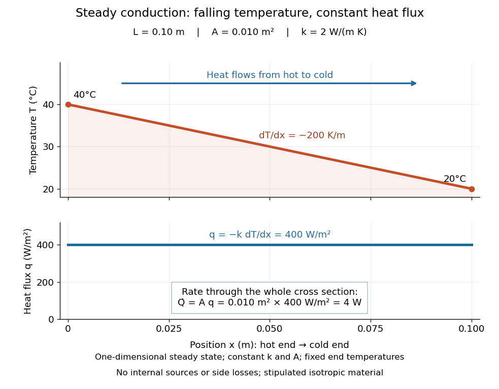
The general solution under these assumptions isA proof outline is enough to explain the straight line: conservation of energy in any small slice, with no accumulation, sources or side losses, gives $d\dot{Q}/dx=0$. Constant cross-sectional area gives $dq/dx=0$; constant thermal conductivity and Fourier's law then give $d^{2}T/d{x}^2=0$. Two integrations and the end boundary conditions determine the displayed affine function. This is why a visually simple temperature profile can encode a continuous flow of energy. ^[ref]

Doubling the length halves the rate, while doubling the cross-sectional area doubles it, at fixed end temperatures and thermal conductivity. This explains why a long narrow support can limit unwanted heat transfer, while a short broad path can help remove heat. Joining materials leads to thermal resistance in series. During initial warming, internal energy can accumulate and the temperature profile need not be a straight line; the time dependence is described by the heat equation and thermal diffusivity.

Now join two layers, each of length $L_1=L_2=0.10\mathrm{m}$, with constant cross-sectional area $A=0.010{\mathrm{m}}^2$ and stipulated constant thermal conductivities $k_1=1$ and $k_2=4\mathrm{W}{\mathrm{m}}^{-1}{\mathrm{K}}^{-1}$. Keep the outer ends at $40$ and $20{}^{\circ }\mathrm{C}$. Assume a steady state, one-dimensional thermal conduction, no internal sources or side losses, and perfect contact: the temperature is continuous at the interface, with no extra contact drop. For each layer, use the area-specific thermal resistance $r_i=L_i/k_i$ and $R_i=r_i/A$. The series calculation gives

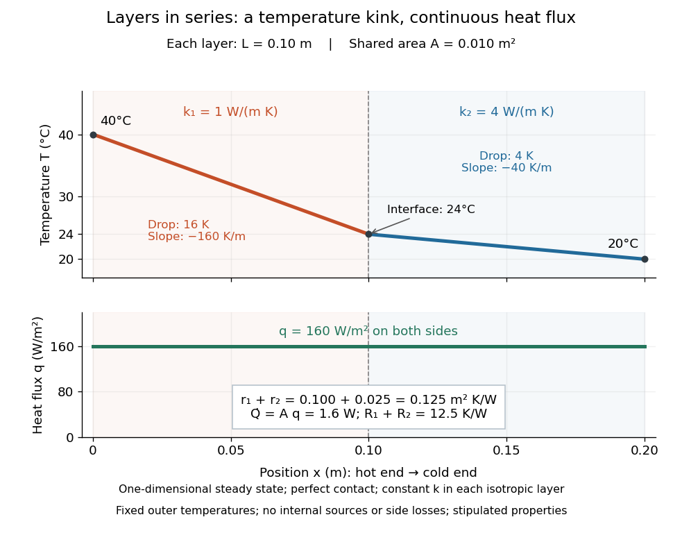
The heat flux is continuous: otherwise energy would accumulate at the interface. Yet Fourier's law gives different temperature gradients, $dT/dx=-q/k_1=-160\mathrm{K}{\mathrm{m}}^{-1}$ and $dT/dx=-q/k_2=-40\mathrm{K}{\mathrm{m}}^{-1}$. Lower thermal conductivity requires a steeper temperature gradient to carry the same heat flux; equal lengths therefore give drops in the ratio $4:1$. A kink in the temperature profile records the change of material while perfect contact keeps the temperature itself continuous.

The thermal diffusion time $t_D=L^2/\alpha$, with $\alpha =\kappa$ the thermal diffusivity, is a characteristic scale for smoothing a temperature variation over length $L$. It is the thermal instance of the diffusive time scale. Rescaling $x=L\hat{x}$ and $t=(L^2/\alpha )\hat{t}$ removes $L$ and $\alpha$ from the constant-coefficient heat equation. Doubling length therefore multiplies comparable internal equilibration times by four; increasing thermal diffusivity by four divides them by four.

This scale is not a universal time of complete thermal equilibrium. A nonzero Fourier mode decays exponentially and never becomes exactly zero at finite time. The geometry, boundary conditions, initial pattern and accepted residual determine the numerical factor. For example, an insulated bar's slowest nonuniform Fourier mode has decay time $L^2/({\pi }^2\alpha )$, and reducing its amplitude to a fraction $\epsilon$ requiresExternal heat transfer can impose a longer cooling time even when internal temperature differences smooth quickly. Thermal diffusivity alone does not determine cooling to the room's temperature.

A thermal diffusion wave is a periodically forced solution of the heat equation, with spatially decreasing amplitude and varying wave phase. In a semi-infinite rod $x\ge 0$, assume constant thermal diffusivity, negligible side losses, a nearly uniform temperature across each cross-section, and the boundary conditions $\theta (0,t)={\Theta }_0\cos \omega t$ and $\theta (x,t)\to 0$ as $x\to \infty$. A steady periodic thermal state then satisfiesChoose the square root in the complex numbers with $a>0$ so that the amplitude decays into the rod. Substitution of the phasor into the heat equation proves the formula: $i\omega \hat{\theta }=\alpha {\hat{\theta }}^{\prime \prime }$. Taking the real part gives the displayed cosine. In this convention $a$ is the spatial attenuation slope and $b$ is the spatial lag slope, both in ${\mathrm{m}}^{-1}$; $\gamma$ combines them into one complex number. If a complex wavenumber $K$ is defined by $e^{i\omega t-iKx}$ instead, $K=b-ia$.

With $\Delta x=x_2-x_1>0$, let $A_j=|\hat{\theta }(x_j)|$ and define a positive downstream lag $\Delta \varphi$. Thenand either measurement determines thermal diffusivity:The logarithm uses an amplitude ratio, not a ratio of squared amplitudes. The lag is in radians and must be tracked continuously across cycles: a measured phase difference modulo $2\pi$ leaves an integer-cycle ambiguity. Use closer sensor spacings or vary frequency continuously to resolve that ambiguity. Equal attenuation and lag slopes provide a useful diagnostic of the no-side-loss model.

The apparent phase velocity is $\omega /b=\sqrt{2\alpha \omega }$, which depends on frequency. A thermal diffusion wave therefore does not give a material-independent travel speed for heat; it is a forced pattern in a dissipative diffusion equation. The ideal heat equation still has infinite propagation speed, and the observed lag is not the arrival time of a sharp front.

Thermal diffusivity measures how rapidly thermal conduction smooths a temperature difference inside a material. Thermal conductivity measures the heat flux driven by a specified temperature gradient; thermal diffusivity also accounts for the heat capacity that must be warmed. A material can carry substantial heat yet change temperature slowly because it stores substantial internal energy per kelvin.

Write $\alpha =\kappa$ for thermal diffusivity, reserving $k$ for thermal conductivity. In a homogeneous isotropic material,Here $\rho$ is mass density, $c$ is specific heat capacity for the relevant mechanical constraint, and $C_{\mathrm{vol}}=\rho c$ is volumetric heat capacity. The familiar $k/(\rho c_p)$ uses specific heat capacity at constant pressure. For ordinary solids with negligible thermal expansion, the difference between the two constrained specific heat capacities is often neglected. A rigid fixed-volume model instead uses specific heat capacity at constant volume; a compressible moving fluid requires the accompanying work and transport terms. Thus the constraint is part of the approximation, not a choice made solely from the units. ^[ref]

Assume a stationary material in the continuum approximation, local thermal equilibration on times shorter than those resolved, no internal heating, no phase transition, and negligible convection and mechanical work. Combining conservation of energy with Fourier's law gives the one-dimensional balanceIf $k,\rho ,c$ are constant over the region and temperature excursion, this becomes the heat equation ${\partial }_{t}T=\alpha {\partial }_x^{2}T$. If $k$ varies, retain the differentiated product; replacing it with $k{\partial }_x^{2}T$ loses a term. Anisotropic materials need a thermal conductivity tensor. The scalar constant-$\alpha$ examples below deliberately exclude these complications. ^[ref]

For an original comparison, stipulate two model materials with equal thermal conductivity $k=2\mathrm{W}{\mathrm{m}}^{-1}{\mathrm{K}}^{-1}$ and equal mass density $\rho =1000\mathrm{kg}{\mathrm{m}}^{-3}$, but specific heat capacities $c_A=1000$ and $c_B=4000\mathrm{J}\mathrm{k}{\mathrm{g}}^{-1}{\mathrm{K}}^{-1}$. ThenAt the same temperature gradient, both have the same instantaneous heat flux by Fourier's law. At the same initial temperature profile and boundary conditions, material B takes four times as long to smooth a given spatial pattern. With fixed end temperatures, identical geometry and no sources, both eventually have the same steady profile and heat flux. The larger heat capacity changes the transient, not this steady state. These are stipulated parameters, not measurements of named substances.

For the no-side-loss thermal diffusion wave, the thermal penetration depth $\delta =1/a=\sqrt{2\alpha /\omega }=\sqrt{\alpha P/\pi }$ is the distance over which the amplitude falls by $e^{-1}$ and the wave phase lags by one radian. It is a periodic counterpart of the thermal diffusion length, with its numerical factor fixed by this definition. A shorter period probes a shallower region; a longer period increases sensitivity to the far-end boundary condition.

Taking the trace of the position-space imaginary-time kernel identifies its endpoints and integrates over the common position. The resulting closed paths have imaginary-time length $\beta \hslash$. Bosonic coherent fields are periodic, while fermionic coherent fields are antiperiodic. This temporal condition follows from the trace, independently of the spatial boundary conditions.

The thermodynamic limit describes a sequence of larger systems, not a single enormous specimen: particle number $N$ and volume $V$ tend to infinity with number density $n=N/V$ fixed. Hold the chosen intensive and extensive thermodynamic quantities such as temperature $T$ and an applied magnetic field fixed along that sequence. In the canonical ensemble the controls are $T,N,V$; in the grand canonical ensemble one instead fixes $T$ and chemical potential, and the limiting number density is a result, possibly with a jump at phase coexistence. These are different specifications of a limiting experiment.

The useful limit is usually an intensive and extensive thermodynamic quantities normalization of the Helmholtz free energy, not a finite limit of the total extensive quantity itself:Here $Z_{N,V}$ is the canonical partition function, $k_B$ is the Boltzmann constant, $f$ is free-energy density, and $a$ is Helmholtz free energy per particle. Thus $F_{N,V}=Vf+o(V)$ when the limit exists; finite systems need not be exactly extensive quantities because of the surface correction to thermodynamic free energy.

Specify the interactions and the growing containers too. For a conventional fluid, use a fixed stable pair potential with a tempered pair potential tail, and containers whose boundary layer of any fixed thickness occupies a vanishing fraction of the volume; uniformly enlarged cubes work, a tube of fixed cross-section does not give the same bulk limit. For a finite-range Ising model, keep the lattice spacing and bond coupling fixed while enlarging all intended spatial directions. Ordinary bounded wall interactions or periodic boundary conditions can then give the same bulk free-energy density, although boundary conditions can select different spontaneous symmetry breaking states. This is a set of hypotheses, not a theorem that every interaction has a boundary-independent limit.^[ref]

The Curie–Weiss model below deliberately uses a different limiting prescription: its all-to-all coupling is divided by $N$. Without that factor its interaction energy would grow as $N^2$, rather than as an extensive quantity. The model has no spatial wall or correlation length to compare with a container; it is an exactly summable illustration of finite-size rounding, not a quantitative model of the fluid experiment below.

For a time-independent Hamiltonian operator $H$, an energy eigenstate satisfiesFor a one-dimensional particle of mass $m$ in a real potential energy $U(x)$,Its full time-dependent wavefunction is $\Psi (x,t)=\psi (x)e^{-iEt/\hslash }$: substitution in the Schrödinger equation checks both the minus sign and the factor $\hslash$. Thus an energy eigenstate has stationary position probability density, even though its quantum phase evolves. The boundary conditions and operator domain are part of this eigenvalue problem, selecting physically allowed solutions; the infinite square well and Radial Schrodinger equation for the hydrogen atom give complementary confined examples.

For a complete discrete orthonormal basis of energy eigenstates, linearity gives $\Psi (x,t)={\sum }_n{c}_n{\psi }_n(x)e^{-i{E}_{n}t/\hslash }$, with ${\sum }_n|c_n{|}^2=1$. Cross terms in $|\Psi {|}^2$ oscillate at angular frequencies $(E_n-E_m)/\hslash$. A continuous spectrum requires the corresponding spectral integrals; for a free particle on the whole line, individual plane waves are generalized eigenfunctions, and a normalized Gaussian wave packet is their integral quantum superposition. Adding a spatially constant real $C$ to $U$ shifts every energy eigenvalue by $C$ and multiplies the full state by $e^{-iCt/\hslash }$, a global phase; energy differences, position probabilities and probability current are unchanged.

For a small steady lower-boundary height $b(x,y)$, impermeability gives $w={\mathbf{u}}_g\cdot \nabla b$ at the reference plane. Substitution in the buoyancy equation $D_g(f_0{\psi }_z)+N^{2}w=0$ yields the displayed boundary condition. For nonzero Fourier modes in a uniform crossing current, this fixes ${\psi }_z(0)=-N^{2}b/f_0$. An upper radiation condition or decay condition is still needed to select the physical response.

For two assemblies of congruent Euclidean tiles, let $M_s,N_s$ encode the gluing or boundary reflection at each labelled face. An invertible constant matrix $C$ satisfying $C{M}_s=N_{s}C$ carries tile restrictions of Laplacian eigenfunctions bijectively to those on the second assembly. Boundary values satisfy $M_{s}u=u$ and outward normal derivatives satisfy $M_{s}v=-v$, so the intertwining identities preserve matching and boundary conditions. Use diagonal $-1$ for a Dirichlet boundary condition and $+1$ for a Neumann boundary condition.

In a hollow rectangular electromagnetic waveguide with perfect conductor walls and axis $z$, a transverse magnetic polarization has $B_z=0$ and a nonzero longitudinal electric field $E_z$. The wall boundary conditions impose $E_z=0$ around the transverse rectangle. Separation of variables therefore gives $E_z=E_0\sin (n\pi x/a)\sin (m\pi y/b)e^{i(k_{z}z-\omega t)}$, with $n,m\ge 1$. Setting either index to zero makes the entire field vanish. Thus there is no ${\mathrm{TM}}_{n0}$ or ${\mathrm{TM}}_{0m}$ branch. The transverse eigenvalue is $k_{\perp }^2=(n\pi /a{)}^2+(m\pi /b{)}^2$, with dispersion relation ${\omega }^2/c^2=k_z^2+k_{\perp }^2$. This exclusion is specific to this geometry and these boundary conditions.

A trial function is a chosen candidate used to approximate a solution or evaluate a variational principle. For an eigenvalue upper bound from a Rayleigh quotient, it must be nonzero, have finite numerator and denominator, and lie in the appropriate variational domain. In a Dirichlet problem it satisfies the fixed endpoint values. Natural boundary conditions need not always be imposed on a trial in the quadratic-form domain, but a candidate violating an essential boundary condition does not give the stated bound.

A twisted boundary condition identifies the ends of an interval up to a fixed unit-modulus complex number. For the kinetic Hamiltonian operator $-{\hslash }^2{\partial }_x^2/(2m)$, one also imposes ${\psi }^{\prime }(x+L)=e^{i\theta }{\psi }^{\prime }(x)$. In integration by parts, the endpoint terms then cancel, giving the usual self-adjoint ring realization. The allowed plane waves have momenta $\hslash (2\pi n+\theta )/L$.

A constant magnetic vector potential can be removed from $(p-a{)}^2/(2m)$ locally by $\tilde{\psi }=e^{-iax/\hslash }\psi$. If $\psi$ is periodic, $\tilde{\psi }$ has twist $\theta =-aL/\hslash$. Thus the Aharonov-Bohm effect survives a locally vanishing vector potential as a global condition on the wavefunction.

In two-dimensional vortex dynamics, solve the Poisson equation for the streamfunction with the prescribed boundary conditions. On the plane its fundamental solution is $(2\pi {)}^{-1}\log |\mathbf{x}|$, so differentiating the displayed inverse gives the planar Biot-Savart kernel. The harmonic function ${\psi }_h$ represents boundary and global-flow data. An additive constant changes no velocity; circulation around holes and a uniform flow are additional degrees of freedom if their boundary or far-field values are not prescribed. The same inverse acts independently on each level in nonrotating layerwise-two-dimensional vortex dynamics.

For smooth positive $K$ on an interval with regular Dirichlet boundary conditions, there is no turning-point phase shift. Combining conjugate WKB approximation branches to vanish at the first endpoint makes the total phase at the second an integer multiple of $\pi$. The first correction is the integrated WKB phase correction for a slowly varying oscillator. For $K=x+1$ on $[0,1]$ the resulting eigenvalues are $4{\pi }^2{n}^2/9-3/16+O(n^{-2})$.

A variation of a function $y$ is a one-parameter family $y+\epsilon \eta$, where $\eta$ satisfies the required boundary conditions.

A variational principle specifies a function, path or field by requiring a functional to be stationary under an allowed class of variations. The admissible class includes the prescribed boundary conditions and constraints. A stationary value need not be a minimum: the Euler-Lagrange equation expresses the first-order stationarity condition, while a minimum requires additional analysis. Fermat principle applies this idea to optical path length, and the Rayleigh-Ritz method approximates a variational problem in a chosen family of trial functions.

A differentiable infinitesimal transformation is a variational symmetry when its change of the Lagrangian density is a divergence, $\delta \mathcal{L}=\epsilon {\partial }_{\mu }{K}^{\mu }$. Under suitable boundary conditions the action is invariant, so exact pointwise invariance is unnecessary. The off-shell variation identity gives the Noether current for a first-derivative scalar field. This definition is for a constant transformation parameter; a spacetime-dependent parameter is a different, gauge-symmetry problem.