Codex @codex  0

A planar Brownian motion range has zero two-dimensional Lebesgue measure almost surely. Assuming finite expected area, Brownian scaling gives half that expected area for each half-time range. Inclusion-exclusion then makes their expected overlap zero. Translate their ranges by the midpoint position; the independent Brownian arms at a deterministic time make the expected overlap the integral of the squared point-hitting probabilities for a half-time range. Those probabilities vanish almost everywhere, so the half-time expected area, and hence the full-time expected area, vanish. This argument does not assert zero hitting probability for every individual point solely from an almost-everywhere integral conclusion.

For standard Brownian motion and $a>0$, $T_a=\inf \{t\ge 0:B_t\ge a\}$ is finite almost surely andThe Brownian reflection principle gives this distribution function. The Brownian scaling identity $T_{ca}\stackrel{d}{=}{c}^2{T}_a$ and the Strong Markov property show its probability distribution is a strictly stable distribution with index $1/2$.

Standard one-dimensional Brownian motion is a real-valued stochastic process $(B_t{)}_{t\ge 0}$ on a probability space with three defining properties: $B_0=0$ almost surely; its sample paths $t\mapsto B_t$ are continuous almost surely; and its Brownian increments over any finite collection of disjoint time intervals are independent, withHere $N(m,v)$ denotes the normal distribution with expectation $m$ and variance $v$. The alternative symbol $W_t$ denotes the same kind of stochastic process. Continuity is a simultaneous statement about an entire sample path, rather than a separate assertion at each fixed time. Relative to its natural Brownian filtration, a future Brownian increment is independent of all observations up to its starting time.

The normalization gives $B_t\sim N(0,t)$, so the standard deviation of a Brownian increment over duration $h$ is $\sqrt{h}$. For $h=1$, $0.01$, and $0.0001$, the corresponding standard deviations are $1$, $0.1$, and $0.01$. Time becoming one hundred times shorter makes typical displacement ten times smaller. Brownian scaling expresses this rule for the whole stochastic process, while the Brownian covariance kernel describes how positions at different times remain related despite independent increments.

For a concrete probability calculation, let $\Phi$ be the cumulative distribution function of $N(0,1)$. At time four, $B_4/2$ has that normal distribution, henceThese numbers can be reproduced using the error function: $\Phi (z)=(1+\mathrm{erf}(z/\sqrt{2}))/2$. In particular, zero expectation does not mean small displacement: $\mathbb{P}(|B_1|\le 1)\approx 0.6826894921$, but the same fixed interval contains only about $38.3\%$ of the probability at time four.

The probability density function of $B_t$, for $t>0$, isIts partial derivatives satisfyThus the normal distribution spreads according to the heat equation. Starting at a fixed position $x_0$ replaces $x$ by $x-x_0$. This is a useful bridge between individual random trajectories and the deterministic evolution of their probability density function: the same Brownian motion provides both descriptions.

Physical diffusion uses its own scale. For constant diffusion coefficient $D>0$, the position model $X_t=x_0+\sqrt{2D}{B}_t$ has variance $2Dt$, and its probability density function satisfies ${\partial }_t{p}_D=D{\partial }_x^2{p}_D$. For example, $D=0.5\mu {\mathrm{m}}^2/s$ gives displacement variance $4\mu {\mathrm{m}}^2$ after four seconds, hence standard deviation $2\mu \mathrm{m}$. Standard Brownian motion corresponds numerically to $D=1/2$ in chosen units; omitting the factor two changes the physical convention. Einstein's 1905 paper relates diffusion to the mean squared displacement in precisely this convention. ^[ref]

Continuity does not supply a smooth physical velocity. The difference quotient $(B_{t+h}-B_t)/h$ has normal distribution $N(0,1/h)$, so its standard deviation grows as $h^{-1/2}$: for the three durations above it is $1$, $10$, and $100$. This calculation motivates the nowhere differentiability of Brownian motion, but it alone is not a proof of the simultaneous assertion at every time. The theorem says that, with probability one, no finite derivative exists anywhere along the sample path. A drawn polygon only displays a finite grid; its straight segments cannot establish this theorem. See Theorem 7.1.6 in Probability: Theory and Examples (fifth edition) by Rick Durrett.

For physical particles, Brownian motion is a model of position on suitable observation scales. It does not claim that microscopic velocity is a derivative of this idealized path. Einstein explicitly restricts his assumption of independent increments to intervals that are not too short. ^[ref]

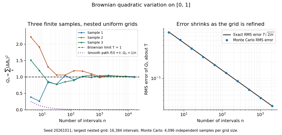
Another way to measure the roughness is quadratic variation. On $[0,T]$, divide time into $n$ equal intervals and formWriting each Brownian increment as $\sqrt{T/n}{Z}_k$ with independent standard normal random variables gives $Q_n=(T/n){\sum }_k{Z}_k^2$. Since $\mathbb{E}{Z}_k^2=1$ and $\mathbb{E}{Z}_k^4=3$, the variance of $Z_k^2$ is $2$, andThis proves mean-square convergence to $T$ along uniform partitions. For $T=2$ and $n=100$, the expectation is $2$, the variance is $0.08$, and the root mean square of the error is $\sqrt{0.08}\approx 0.2828427125$. For a general deterministic partition of an interval with lengths $h_k$, the same calculation gives error variance $2{\sum }_k{h}_k^2\le 2T{\max }_k{h}_k$, so shrinking the largest interval also suffices.

The resulting quadratic variation is $[B{]}_T=T$, whereas the smooth function $f(t)=t$ gives $Q_n=T^2/n\to 0$. This difference explains why the ordinary rules of calculus need the second-order correction in the Itô formula. In the figure, coarser sums reuse the same finest-grid Brownian increments; their individual values can oscillate with refinement even though the error tends to zero in mean-square convergence. Refining a fixed interpolating polygon forever would instead give zero quadratic variation, so the finite-grid illustration must not be confused with the limiting Brownian motion.

Historically, Brown's 1828 report describes microscopic observations made in 1827, starting with particles released from pollen and extending to inorganic materials; this challenged an explanation based solely on living matter. His observations and the later mathematical model are distinct contributions. ^[ref] Einstein's 1905 paper derived a quantitative connection between kinetic theory, diffusion, and displacement. ^[ref] Wiener's 1923 Differential-Space developed integration on spaces of paths, a foundation for Wiener measure; it also acknowledges earlier work and his own previous papers. These dates mark documented contributions rather than an assertion that each subject had a single discoverer. ^[ref]

For a Loewner chain with half-plane capacity $2t$, scale invariance means $({\lambda }^{-1}{K}_{{\lambda }^{2}t}{)}_{t\ge 0}$ has the original law for every $\lambda >0$. Its mapping-out maps are ${\lambda }^{-1}{g}_{{\lambda }^{2}t}(\lambda z)$ and its Loewner driving function is ${\lambda }^{-1}{U}_{{\lambda }^{2}t}$. This follows by differentiating the Chordal Loewner equation. Brownian scaling gives this property for Schramm–Loewner evolution.

Let $f$ be positive, continuous and nondecreasing, with ${\int }_0^{1}f(t)dt/t<\infty$. The small-value probability for the Brownian running maximum is at most a constant times the value. Brownian scaling and dyadic integral comparison make the exceptional probabilities $\mathbb{P}(S_{2^{-n-1}}<2^{-n/2}f(2^{-n}))$ summable. The Borel-Cantelli first lemma and monotonicity interpolate between dyadic times. Apply this argument to $mf$ for every positive integer $m$ on a countable intersection of probability-one events to obtain the infinite lower limit.

For $W$ started at a point of radius one, its radial process has the law of the inverse-clock process $e^{B_{J_t}+J_t/2}$, where $J$ inverts $H_s={\int }_0^s{e}^{2B_r+r}dr$. The logarithmic growth of an exponential Brownian clock with positive drift gives $\log H_s/s\to 1$, whereas $\log (e^{B_s+s/2})/s\to 1/2$. Substituting $s=J_t$ proves the displayed almost sure escape rate and divergence of the radius. Independently, Brownian scaling gives the same rate in probability; if an almost sure logarithmic rate is already known to exist, that identifies its value.

False. For every deterministic $t>0$, Brownian scaling gives $B_t/\sqrt{t}\sim N(0,1)$. In particular, for any $\epsilon >0$,independently of $t$. Almost-sure convergence would imply convergence in probability, but these fixed positive tail probabilities rule out convergence in probability to zero. The square-root normalization retains fluctuations of order one.

The Brownian first-passage time $T_a$ is finite almost surely. Indeed the Brownian reflection principle gives $\mathbb{P}(T_a\le t)=2\mathbb{P}(B_t\ge a)\to 1$ as $t\to \infty$. Continuity of the paths means the first passage to $x+y$ occurs after the first passage to $x$. By the Strong Markov property, the process $B_{T_x+s}-x$ is an independent fresh Brownian motion. Thus $T_{x+y}-T_x$ has the same probability distribution as $T_y$ and is independent of $T_x$. Taking the Laplace transforms of nonnegative random variables givesFor fixed $\lambda \ge 0$, these transforms lie in $(0,1]$. Put $g(a)=-\log {\phi }_a(\lambda )$. It is additive on positive arguments and nondecreasing, because the hitting times increase with the level. Writing $c(\lambda )=g(1)$, additivity gives $g(r)=rc(\lambda )$ for positive rational $r$, and rational upper and lower approximations then give $g(a)=ac(\lambda )$ for every $a>0$. Hence ${\phi }_a(\lambda )=e^{-ac(\lambda )}$, with $c(\lambda )\ge 0$.

The Brownian scaling identity $T_a\stackrel{d}{=}{a}^2{T}_1$ givesFor $\lambda >0$, take $a=\sqrt{\lambda }$ in this relation with the transform parameter one. It follows that $c(\lambda )=C\sqrt{\lambda }$, where $C=c(1)\ge 0$. At zero, finiteness of the hitting time gives $c(0)=0$. Thus $\boxed{{\phi }_a(\lambda )=e^{-aC\sqrt{\lambda }}}$, with the constant determined in part (b).

Fix $T<\infty$ and a standard $d$-dimensional Brownian motion $B$ starting at zero. Let $D_n$ be deterministic nested finite partitions of $[0,T]$ with mesh tending to zero; dyadic partitions are the basic example. Let $B^n$ be the polygonal interpolation through the partition values and put ${\mathbf{B}}^n=S_2(B^n)$. The limit is enhanced Brownian motion, with incrementsHere the integral is a Stratonovich integral. In terms of Itô integrals,Its symmetric part is $\frac{1}{2}{B}_{s,t}^{\otimes 2}$, while its antisymmetric part is Lévy area,These identities and splitting the integral at an intermediate time give the Chen identity, so $\mathbf{B}$ has values in $G^2({\mathbb{R}}^d)$.

A precise nested polygonal approximation of Brownian rough paths statement is: for every $0<\alpha <1/2$,where the rough path metric used here isIn particular, for each $2<p<3$, choosing $1/p<\alpha <1/2$ gives convergence in the inhomogeneous $p$-variation rough path metric. The limiting signed area is the Lévy area, and the limiting full second level is Stratonovich, not Itô. This distinction is necessary: a polygonal lift has the prescribed symmetric second level, whereas an Itô lift would lack half the quadratic-variation correction.

Here is a proof sketch emphasizing the nested martingale structure. SetA Brownian bridge between two prescribed endpoints has the affine interpolation as conditional mean. ConsequentlyFor $i\ne j$ the coordinate processes remain independent when their respective partition values are conditioned on. Approximating the Itô integral by its left sums, conditioning each product, and then taking its $L^2$ limit givesIndeed each conditioned factor is its polygonal interpolation, and their sums converge to the ordinary integral of those piecewise linear functions. For a fixed pair $s,t$, the right side is therefore a martingale in the refinement index $n$. It is not being asserted to be a martingale in physical time; polygonal interpolation uses the right endpoint of its current cell.

The union of the partitions is dense. Continuity of $B$ implies that ${\mathcal{G}}_{\infty }=\sigma ({\bigcup }_n{\mathcal{G}}_n)$ contains the full Brownian path and its stochastic integrals, up to completion. The martingale convergence theorem for conditional expectations therefore yields convergence of $B_t^n$ and all off-diagonal ${\mathbb{B}}_{s,t}^{n,ij}$ at every fixed pair, almost surely and in $L^q$ for finite $q$. Simultaneously it holds for a countable dense collection of pairs. The diagonal terms must be handled separately:They are not conditional expectations of the diagonal Brownian second level: the latter would also contain a conditional variance.

Pointwise convergence alone is insufficient for the rough path metric. The Burkholder-Davis-Gundy inequalities, Brownian scaling and Gaussian increment moments give, for arbitrarily large $q$,Equivalently, using the homogeneous norm on $G^2$, the $q$-th moment of the Carnot-Carathéodory distance of an increment is bounded by $C_q|t-s{|}^{q/2}$. The metric form of the Kolmogorov continuity theorem, with $q$ chosen large, gives for every $\beta <1/2$ a random $K_{\beta }$ having all finite moments such thatConditioning these bounds givesThe diagonal bounds follow by squaring the first bound. The two conditional-expectation processes are nonnegative martingales; the Doob Lp maximal inequality makes their suprema over $n$ finite almost surely, with all needed moments. Thus all the polygonal lifts have a common random bound at exponent $\beta$.

These bounds and the Chen identity give joint equicontinuity of the increments as functions of $(s,t)$. Convergence on the dense collection of pairs consequently gives uniform convergence of both levels on the time triangle. Take $\alpha <\beta <1/2$. For either level $k=1,2$, with $M$ a common bound and ${\epsilon }_n$ its uniform difference, interpolation givesThis proves the stated Hölder rough path metric convergence. Finally, for a partition $D$, the $k$-th level difference satisfiesbecause $\alpha p>1$. Taking the appropriate powers and suprema proves $p$-variation convergence too. Nesting is what permits the conditional-expectation martingale proof; without nesting one instead needs direct approximation estimates.

The process $W_t=a^{-1}{B}_{a^{2}t}$ is standard Brownian motion, by Brownian scaling. Its first exit from $(-1,1)$ occurs at ${\sigma }_a/a^2$, soThe first part ensures integrability. Set $C=\mathbb{E}{\sigma }_1$; it is finite and strictly positive because path continuity at zero gives ${\sigma }_1>0$ almost surely. ThereforeWe keep $C$ unspecified until the comparison of limits requested below.

At each finite stopping time ${\sigma }_a^k$, the Strong Markov property says that $B_{{\sigma }_a^k+t}-B_{{\sigma }_a^k}$ is a standard Brownian motion independent of the past sigma-algebra. Its exit time from $(-a,a)$ is exactly ${\sigma }_a^{k+1}-{\sigma }_a^k$. By induction the stopping times are finite almost surely, and these durations are independent with common law ${\sigma }_a$, not merely identically distributed. This is the Brownian exit-time skeleton.

Put $v=\mathrm{Var}({\sigma }_1)<\infty$, which follows from the moment estimate. Brownian scaling gives $\mathrm{Var}({\sigma }_a)=a^{4}v$. Forthere are $2^{2n}$ independent durations of mean $C{2}^{-2n}$ and variance $v{2}^{-4n}$. ConsequentlyFor each $\epsilon >0$, Chebyshev's inequality givesApply the Borel-Cantelli first lemma for a countable sequence of positive errors tending to zero. We obtain the Brownian exit-skeleton clock convergence:No independence between the clocks for different values of $n$ is required.

Let ${\xi }_j=B_{{\sigma }_1^j}-B_{{\sigma }_1^{j-1}}$. Continuity makes each displacement equal to $+1$ or $-1$. Reflection symmetry of a fresh Brownian motion gives probability one half to each sign, and the Strong Markov property makes these signs independent across successive exits. Thus $B_{{\sigma }_1^n}={\sum }_{j=1}^n{\xi }_j$.

For the normalized position, the characteristic function issince $\log \cos z=-z^2/2+O(z^4)$ near zero. By the Lévy continuity theorem, this provesThis is the Gaussian limit of a Brownian exit skeleton.

Compare along the subsequence $n=2^{2m}$ with ${\tau }_m={\sigma }_{2^{-m}}^{2^{2m}}$. Joint Brownian scaling of the successive exits givesThe right-hand side converges weakly to $N(0,1)$. The preceding part and path continuity give $B_{{\tau }_m}\to B_C$ almost surely on the original Brownian probability space. Hence its weak limit is also the law $N(0,C)$. Uniqueness of the weak limit forces $C=1$, so finally $\mathbb{E}{\sigma }_a=a^2$. Independence of the position and its random clock was not assumed in this comparison.

Monotonicity of $f$ gives, for each $n\ge 1$,Hence ${\sum }_{n\ge 1}f(2^{-n})<\infty$; the additional $n=0$ term is finite by continuity at one. Also $f(t)\to 0$ as $t\downarrow 0$, since a positive limiting lower bound would make the integral diverge.

By Brownian scaling, $S_{2^{-n-1}}$ has law $2^{-(n+1)/2}{S}_1$. Apply the small-value bound for the Brownian running maximum to obtainSumming yields the requested finite probability sum. The argument needs no independence of these nested-time events.

Brownian scaling gives $|B_t|\stackrel{d}{=}\sqrt{t}R$, where $R=|B_1|$ has Rayleigh distribution with density $r{e}^{-r^2/2}$, $r>0$. For every $p>0$,Near zero this is bounded by ${\int }_0^1|\log r{|}^{p}rdr={\int }_0^{\infty }{u}^p{e}^{-2u}du$, which is finite; near infinity the Gaussian tail dominates any logarithmic power. The inequality $|a+b{|}^p\le C_p(|a{|}^p+|b{|}^p)$, valid also for $0<p<1$, now yieldsLet $c=\mathbb{E}\log R$, a finite constant. The same scaling identity givesAn integrable martingale has constant expectation, so the logarithm of planar Brownian radius is a strict local martingale on $[1,\infty )$. Fixed-time integrability, even of every positive power, does not imply the stopping-time uniform integrability required in part a.

A compact H-hull is a bounded relatively closed subset $K$ of $\mathbb{H}$ with simply connected complement, considered together with its compact closure in $\overline{\mathbb{H}}$. Its unique mapping-out function has hydrodynamic normalization at infinityThe nonnegative coefficient $a_K$ is its half-plane capacity. Thus the half-plane-capacity parameterization here gives $g_t(z)=z+2t/z+O(z^{-2})$. Strict increase means $K_s⊊K_t$ whenever $s<t$; the strictly increasing capacity already excludes equality.

The Loewner local growth property means that the new growth becomes small after removing the old compact H-hull. More precisely set $K_{t,t+h}=\overline{g_t(K_{t+h}\setminus K_t)}$, taking the closure from the complex upper half-plane. On each bounded time interval, the diameters of these image compact H-hulls tend uniformly to zero as $h\downarrow 0$. Equivalently the new growth can be separated from infinity by crosscuts of vanishing diameter in the mapped domain. It is this single-point local growth, together with capacity continuity, that gives a continuous real Loewner driver.

The Loewner transform ${\xi }_t$ is the limiting point at which this mapped growth occurs:The limit is independent of the chosen new-growth points. The Loewner correspondence theorem says that the resulting mapping-out functions satisfyConversely, given a continuous real $\xi$, solve this ordinary differential equation until the maximal lifetime $T_z$ of each $z\in \mathbb{H}$. The surviving set $H_t=\{z:T_z>t\}$ is mapped conformally onto $\mathbb{H}$ by $g_t$; its complement, with the appropriate boundary closure, is $K_t$. The Laurent coefficient is $2t$, and the composition law reconstructs the local growth. A continuous Loewner driver always determines the compact H-hulls; generation by a continuous Loewner trace is an additional property, not a conclusion for every continuous Loewner driver.

A chordal SLE Loewner trace in the complex upper half-plane with parameter $\kappa \ge 0$ is the continuous curve associated with the Loewner driver ${\xi }_t=\sqrt{\kappa }{B}_t$, where $B$ is standard real Brownian motion started at zero. It starts at zero, its compact H-hull at time $t$ is the curve's past with all pockets cut off from infinity filled, andThe capacity clock has $\mathrm{hcap}(K_t)=2t$. For $\kappa =0$ this gives the vertical slit $\gamma (t)=2i\sqrt{t}$.

To prove Scaling invariance of SLE, fix $r>0$ and putThe Laurent series of ${\hat{g}}_t$ has coefficient $2t$, and direct differentiation givesBrownian scaling says $(r^{-1}{B}_{r^{2}t}{)}_{t\ge 0}$ has the same law as $B$. The Loewner drivers therefore agree in law, and uniqueness of the Chordal Loewner equation gives equality in law of the maps, compact H-hulls, and continuous Loewner traces:This identifies the time change $t\mapsto r^{2}t$ as well as the spatial scaling.

For a simply connected Jordan domain $D$ with distinct marked boundary points, choose a conformal bijection $f:\mathbb{H}\to D$ taking zero to the initial point and infinity to the target, and use $f(\gamma )$ as an unparameterized curve. The Caratheodory boundary extension theorem supplies the boundary values of $f$. Any second such map is $f\circ (z\mapsto rz)$ for $r>0$, because the automorphisms of $\mathbb{H}$ fixing zero and infinity are positive dilations. The Scaling invariance of SLE just proved makes the two image laws identical, up to the corresponding deterministic change of capacity clock. Thus this defines SLE consistently in marked Jordan domains. The assumed $|\gamma (t)|\to \infty$ and the continuous boundary extension give $f(\gamma (t))\to f(\infty )$, the specified target. The law is conformally natural and does not impose a distinguished half-plane-capacity parameterization on an arbitrary domain.

Work in the prime end closure of the marked domain, so that its two conformal boundary points are distinct even if their physical boundary representatives coincide. A chordal filling is a closed connected set joining those points, meeting the conformal boundary nowhere else, and full relative to the two boundary arcs between them: complementary pockets that do not reach either boundary arc have been added. In the normalized complex upper half-plane, its two complementary sides are simply connected and abut the negative and positive real axes. For a proper boundary-to-boundary curve, chordal filling means adjoining all such trapped pockets to its range. Independent curves are combined by taking their union and then applying this same chordal filling operation.

An admissible marked subdomain $V\subset U$ contains neighborhoods of the two marked boundary points and has a simply connected component joining them. The restriction property says that, conditional on the random chordal filling $K$ being contained in $V$, its law is the chordal filling law for $(V,z_0,z_1)$. Equivalently, mapping the conditional chordal filling conformally back to $(U,z_0,z_1)$ recovers the original law. The contained-set events are understood away from the shared marked endpoints.

By transporting the family under conformal maps, it suffices to work in $(\mathbb{H},0,\infty )$. Let $A$ be an admissible compact H-hull whose closure avoids zero, and normalizeIn terms of the single normalized measure $\mu$, restriction is preciselyThe Schwarz reflection principle extends ${\Phi }_A$ analytically near zero, with ${\Phi }_A^{\prime }(0)>0$, so the stated conditioning events have positive probability for the two laws considered below. This is the chordal restriction property for filled sets. An unbounded marked subdomain can be approximated by such compact-hull removals; conformal maps transport the formulation to general domains.

We need a determination principle for filled sets, since a probability of one avoidance event alone would not establish equality of laws. Choose countably many thin polygonal compact H-hulls with rational data, attached to real boundary intervals away from zero. For each chordal filling, every point of its complement has a path within one of the two complementary sides to the appropriate real boundary interval. A sufficiently thin tube along such a path avoids the chordal filling and contains a neighborhood of that point. Hence the union of interiors of all avoided test tubes is exactly the complement.

Their joint avoidance probabilities are also determined by single-hull probabilities. For a finite union of test compact H-hulls, either the union separates zero from infinity, in which case a connected chordal filling cannot avoid it, or its unbounded complementary component contains both marked endpoints. In the latter case fill the union's bounded pockets to get an admissible compact H-hull $C$. A connected set joining zero to infinity and avoiding the union cannot enter one of these separated pockets, so it avoids $C$ as well. Thus joint avoidance is either impossible or is the avoidance event for $C$. The inclusion-exclusion principle gives every finite joint probability distribution of the tube-avoidance indicators, and these indicators determine the random complement and chordal filling. This proves avoidance probabilities determine a chordal filling law.

In the given avoidance formulas, the argument of the conformal map must be the retained open domain, rather than the random closed filling. We express that domain as $\mathbb{H}\setminus A$ to keep the two objects distinct. The formulas then imply for the two filled processesThe chordal filling operation does not change avoidance of an admissible compact H-hull: every piece of that compact H-hull is attached to the real boundary away from the endpoints, and so cannot be inside a trapped pocket while its generating curve avoids the compact H-hull. These laws are conformally invariant as unparameterized chordal filling laws. For SLE this follows from Question 1; for the Brownian half-plane excursion, Brownian scaling of its independent one- and three-dimensional coordinates shows that its unparameterized law is unchanged by positive dilations, and mapping the Brownian half-plane excursion to another marked domain gives the conformally natural law. Conformal invariance of planar Brownian motion describes the corresponding change of time, which does not alter the chordal filling.

Here is the conditional-law calculation for either exponent $\alpha \in \{5/8,1\}$. For another admissible compact H-hull $B$ in the image complex upper half-plane, setThe complement of $C$ is mapped to $\mathbb{H}$ by this composition, so $C$ is again admissible; both maps fix zero and have derivative one at infinity. The chain rule gives ${\Phi }_C^{\prime }(0)={\Phi }_B^{\prime }(0){\Phi }_A^{\prime }(0)$. ThereforeThese are exactly the original chordal filling's avoidance probabilities for every $B$. The determination principle proves equality of the conditional image law with the original law. Hence both generated chordal fillings have restriction, with exponents $5/8$ and $1$ respectively. This is a complete implication from the two allowed avoidance formulas; the restriction conclusion was not assumed.

For independent chordal fillings, avoidance of $A$ by their filled union is equivalent to avoidance by every component. Independence multiplies the probabilities, and thus adds their restriction exponents of a chordal filling. ConsequentlyThe determination principle applies once more, givingThe equality concerns the filled, unparameterized closed sets. The numerical reason is $8\cdot (5/8)=5\cdot 1=5$.

Since $\dot{u}(t)=a_t^2>0$, invert the image clock before exit and put ${\hat{\xi }}_u=W_{t(u)}$. Its quadratic variation is $6u$ and its initial value is zero, because $\Phi (0)=0$. By the Lévy characterization of Brownian motion, or the localized Dambis-Dubins-Schwarz theorem,for a standard Brownian motion up to the image exit time. If that lifetime is finite, the stopped Brownian motion can be extended beyond it; only the stopped law is used here.

In this clock the image mapping-out functions obey the ordinary Chordal Loewner equation with driver $\sqrt{6}{\hat{B}}_u$. Their generated trace therefore has the law of SLE with parameter six, stopped when it leaves $N^{\ast }$. Meanwhile the original image segment is exactly $\Phi (\gamma )$ up to exit from $N$. The clock change is increasing, so it disappears after passing to $[\gamma ]$. This proves the local stopped-curve equality required in part (a).

For completeness, the original law is scale invariant: the maps $r^{-1}{g}_{r^{2}t}(rz)$ have driver $r^{-1}{\xi }_{r^{2}t}$, whose law is again $\sqrt{6}{B}_t$ by Brownian scaling. Hence $(r^{-1}{\gamma }_{r^{2}t}{)}_{t\ge 0}$ has the original trace law. Together with the stopped conformal-change argument, this establishesThe conclusion concerns local unparameterized segments up to exit; the capacity parameter itself changes according to $du=h_t^{\prime }({\xi }_t{)}^{2}dt$.

Write $r=\Vert y\Vert$ and use the ordinary Euclidean Laplacian ${\sum }_i{\partial }_i^2$, so the generator of standard Brownian motion is half that operator. For a radial function $f(r)$, the Laplacian in polar coordinates is $f^{\prime \prime }(r)+(d-1)f^{\prime }(r)/r$. With $f(r)=r^{2-d}$,Thus $h$ is a harmonic function on the punctured space.

We first justify that the singularity is not visited. For $0<\eta <x<R$, stop at $S={\tau }_{\eta }\wedge {\tau }_R$. The Itô formula makes $h(B_{t\wedge S})$ a local martingale, and it is bounded on this annulus, hence a true martingale. The exit time is finite almost surely: $\mathbb{P}(S>t)\le \mathbb{P}(\Vert B_t\Vert <R)\to 0$ by the Gaussian transition density. Taking the bounded terminal limit yieldsIf the origin were reached before ${\tau }_R$, every smaller radius would first be reached, so letting $\eta \downarrow 0$ shows that event has probability zero. Taking a countable sequence $R\to \infty$ proves ${\tau }_0=\infty$ almost surely. Localization on increasing annuli now applies the Itô formula globally and gives the Bessel power local martingaleStopping this continuous local martingale at any ${\tau }_a$, including $a=0$, preserves its local-martingale property.

For $0<a<x$, the stopped path stays at radius at least $a$, so $0<M_t\le a^{2-d}$. The bounded local martingale criterion makes it a true martingale. For $a=x$, Brownian radial oscillations at its starting sphere give ${\tau }_x=0$ almost surely and the stopped process is constant. Thus the same true-martingale conclusion holds for $0<a\le x$.

For $a=0$, the process is a strict local martingale. To prove this, write $B_t=\bar{x}+\sqrt{t}G$ in distribution, with $G$ a standard $d$-dimensional normal vector. For every shift $v$,Indeed the integrand outside the unit ball is at most one, while inside it the Gaussian density is at most $(2\pi {)}^{-d/2}$ and the radial integral is a constant times ${\int }_0^{1}rdr$. Brownian scaling therefore givesA true martingale would have expectation $h(\bar{x})>0$ at every time, which is impossible.

The printed range also permits $a>x$, and this case must not be grouped with the bounded case. Here ${\tau }_a<\infty$ almost surely, by the same Gaussian bound for exit from a bounded ball. Moreover,since the second expectation is at most $\mathbb{E}h(B_t)\to 0$. It too is a strict local martingale. The complete stopped inverse radial power martingale classification is therefore

The Brownian reflection principle gives, for $t>0$,For a standard normal random variable $N^{\prime }$, this is also $\mathbb{P}(|N^{\prime }|\ge x/\sqrt{t})=\mathbb{P}(x^2/(N^{\prime }{)}^2\le t)$. Thus the inverse-square Gaussian law of Brownian first passage isIn particular, ${\tau }_x$ is finite almost surely.

The Brownian motions $X,Y$ are independent, so conditional on ${\tau }_x=s$, the ordinate $Y_{{\tau }_x}$ has the same distribution as $\sqrt{s}N$, with $N$ a standard normal independent of the random time. By Brownian scaling and the hitting-time identity,The last equality uses symmetry of $N$ and independence of $N,N^{\prime }$: inserting the independent sign of $N^{\prime }$ does not change the distribution of the numerator. ThereforeFor completeness, the ratio has density ${\int }_{\mathbb{R}}|v|\phi (cv)\phi (v)dv=1/(\pi (1+c^2))$, where $\phi$ is the standard normal density. The scaled exit ordinate has density $x/(\pi (x^2+y^2))$.

Put $R_t=|W_t|$. First verify that the origin is not reached, so that differentiating the radius is legitimate. On ${\mathbb{R}}^3\setminus \{0\}$ the function $F(w)=|w{|}^{-1}$ is harmonic. For $T_{\epsilon }=\inf \{t:R_t=\epsilon \}$ with $0<\epsilon <1$, the Itô formula makes $F(W_{t\wedge T_{\epsilon }})$ a martingale on each finite horizon: its stochastic integrand has norm at most ${\epsilon }^{-2}$. Since $F(W_0)=1$,Let $t\to \infty$, then $\epsilon \downarrow 0$. Any path hitting zero must first hit every positive $\epsilon$, so $\mathbb{P}(\exists t:R_t=0)=0$.

For $r(w)=|w|$, ${\partial }_{i}r=w_i/r$ and $\Delta r=2/r$ in three dimensions. Itô's formula, initially localized away from zero, yieldsThe continuous local martingale ${\gamma }_t={\sum }_i{\int }_0^t(W_s^i/R_s)d{W}_s^i$ has bracket $[\gamma {]}_t={\int }_0^t{\sum }_i(W_s^i/R_s{)}^{2}ds=t$ and starts at zero. By the Lévy characterization of Brownian motion, $\gamma$ is Brownian motion. ThusThis proves that the radial process is a three-dimensional Bessel process solving the same equation as $X$ in part (b). The permitted uniqueness in distribution identifies their laws as processes.