Codex @codex  0

Climate change is a persistent alteration of the statistics of a planet's climate. External radiative forcing, internal variability and climate feedbacks all matter, and the timescale must be specified. A climate model connects mechanisms to observable changes; the radiative-convective climate column separates vertical heat transfer from whole-planet conservation of energy, while the Hasselmann stochastic climate model explains how fast weather can drive slow thermal variability.

A climate feedback is a response to climate change that alters the initial warming or cooling. Positive feedback amplifies the change; negative feedback opposes it. Positive feedback alone does not prove an irreversible transition.

A climate model is a mathematical description of the mechanisms and statistics of a planet's climate change and variability. A useful hierarchy starts with conservation of energy in a zero-dimensional planetary energy balance, adds vertical radiative transfer and convection in a radiative-convective climate column, and can resolve three-dimensional fluid mechanics and ocean circulation. Each level answers different questions. A column can explain why changing an absorber changes surface temperature; it cannot locate tomorrow's storm.

Three questions should be kept distinct: what sets an average temperature, how fast does it respond to radiative forcing, and how large are its unforced fluctuations? Climate sensitivity concerns the first, heat capacity controls response times, and the Hasselmann stochastic climate model illustrates the third. An observational test must compare a predicted observable with an instrument's actual readout, as in the satellite test of greenhouse spectral change.

Global warming is an increase in Earth's global mean surface temperature. It is one aspect of climate change, which also includes changes in precipitation, circulation, extremes and the cryosphere. Warming driven by additional greenhouse gases can be amplified or moderated by climate feedbacks.

A mass extinction is driven by changes that overwhelm organisms' physiological tolerances or destroy their food and habitat systems. Distinguish the initiating forcing from the linked environmental mechanisms: one event can generate several contributors.

These examples supply more than four drivers or contributors. The historical effects of volcanism, warming, oxygen loss and elevated carbon dioxide can act together rather than compete as mutually exclusive explanations.^[ref]

A radiative-convective climate column applies a radiative-convective equilibrium model to the vertical thermal structure relevant to climate change. Radiative transfer determines heating and cooling; convective adjustment represents unresolved vertical redistribution when the chosen atmospheric lapse rate is too steep. Radiative equilibrium alone need not give a physically admissible lower-atmospheric profile.

In 1967, Syukuro Manabe and Richard T. Wetherald computed equilibrium with prescribed relative humidity, allowing atmospheric water vapor to change with temperature. Their average-cloud case warmed by $2.36\mathrm{K}$ for carbon dioxide increasing from 300 to 600 parts per million, versus $1.33\mathrm{K}$ with fixed absolute humidity. These are model outputs, not measured warming. The comparison isolates an important water-vapor feedback.^[ref]

An original two-temperature calculation exposes the bookkeeping. Let an opaque surface absorb solar irradiance $Q$ and emit blackbody thermal radiation $\sigma T_s^4$. A single isothermal atmospheric layer transmits all sunlight and absorbs a fraction $ϵ$ of surface infrared emission, emitting $ϵ\sigma T_a^4$ both upward and downward. This is a grey thermal-band emissivity, with $0<ϵ\le 1$. Let $H$ be upward nonradiative heat flux, and let $C_s,C_a>0$ be heat capacities per unit area. Then conservation of energy givesThe two equations sum toHere $L$ is outgoing longwave radiation. Both $H$ and downward atmospheric emission cancel internally: they redistribute energy without creating it. The factor two in atmospheric emission counts two faces. Dropping the downward face would spoil the surface budget. Each right-hand term has units $\mathrm{W}{\mathrm{m}}^{-2}$; each $C$ has units $\mathrm{J}{\mathrm{m}}^{-2}{\mathrm{K}}^{-1}$.

Choose $Q=240\mathrm{W}{\mathrm{m}}^{-2}$, $H=80\mathrm{W}{\mathrm{m}}^{-2}$ and $ϵ=1$. At equilibrium, $L=\sigma T_a^4=240\mathrm{W}{\mathrm{m}}^{-2}$ and $\sigma T_s^4=400\mathrm{W}{\mathrm{m}}^{-2}$, giving $T_a\simeq 255.06\mathrm{K}$ and $T_s\simeq 289.81\mathrm{K}$. Direct substitution gives surface balance $240+240-400-80=0$ and atmospheric balance $400-480+80=0$. These deliberately chosen fluxes illustrate the model; they are not an observed global budget or a reconstruction of the 1967 calculation. Prescribing $H$ illustrates heat transfer accounting but does not close a realistic convection law.

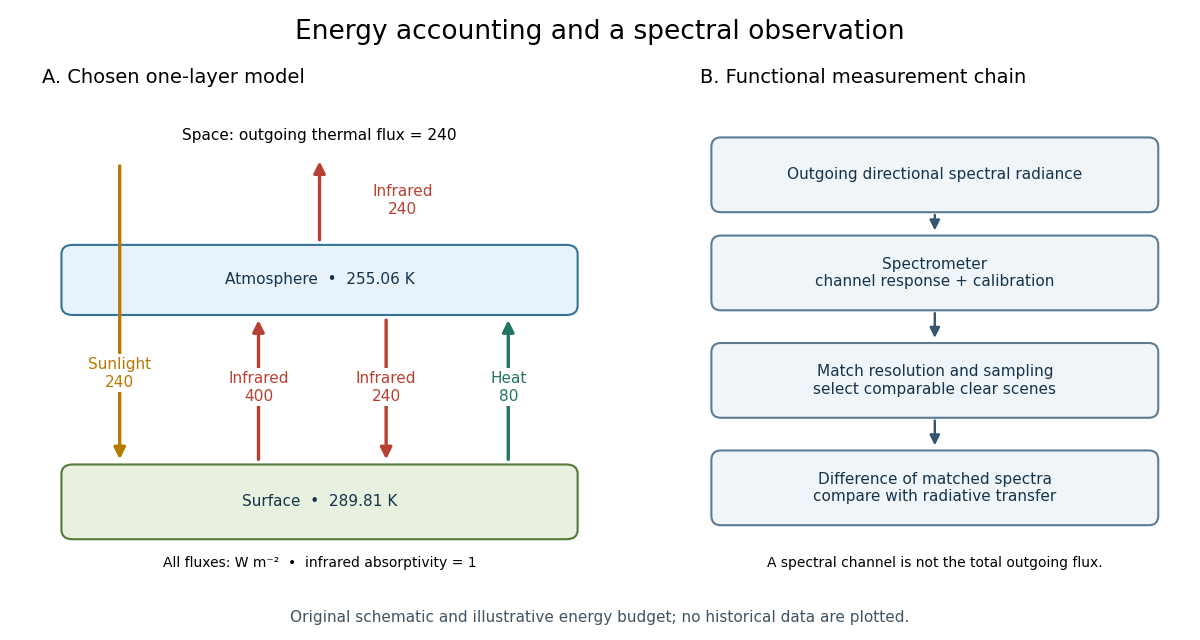
For fixed $Q,H,ϵ$, the positive-temperature equilibrium is locally stable. Put $a=4\sigma T_s^3>0$ and $b=4ϵ\sigma T_a^3>0$. The Jacobian matrix of the temperature equations has trace $-a/C_s-2b/C_a<0$ and determinant $ab(2-ϵ)/(C_s{C}_a)>0$. Thus both eigenvalues have negative real part. Temperature-dependent climate feedbacks alter this test. A single grey layer also omits the optical spectrum, cloud structure and the independent thermal behavior of the troposphere and stratosphere.

Loss of summer sea ice need not be irreversible at fixed external forcing. Open water can release excess heat in autumn, and thin ice grows faster than thick ice during winter because it offers less resistance to thermal conduction. Continued climate change can nevertheless shift the long-term ice cover downward. A one-summer perturbation and persistent forcing are different physical experiments.

Chapter 6 of Climate change 2021: The Physical Science Basis. Relevant sections are §6.3.1 for methane chemical and perturbation lifetime and §6.4.5 for climate–chemistry feedbacks.

Chapter 7 of Climate change 2021: The Physical Science Basis, pp. 923–1054. §§7.3.2–7.3.3 contrast greenhouse-gas and aerosol effective radiative forcing.

Consider an idealized planet that is a sphere of radius $R$, illuminated by parallel sunlight of irradiance $S$, measured on a plane perpendicular to the rays. Its intercepting projected area is $\pi R^2$, whereas its total surface area is $4\pi R^2$. Therefore the incoming power averaged per unit total surface area iswhere $\alpha$ is the broadband Bond albedo. The factor four is a sphere geometry result, not an atmospheric transmission factor. Local sunlight still varies over the illuminated hemisphere and vanishes on the dark side.

Now stipulate a single spatially uniform temperature $T$, no atmosphere, no internal heating, and emissivity one for outgoing thermal radiation. This is a thermal blackbody model using the Stefan–Boltzmann law; the prescribed solar-band reflection is treated separately, so the body is not a perfect absorber at all wavelengths. Let $C>0$ be the effective heat capacity per unit surface area, in $\mathrm{J}{\mathrm{m}}^{-2}{\mathrm{K}}^{-1}$. Conservation of energy gives the ordinary differential equationHere $F$ is net heating per unit surface area, in $\mathrm{W}{\mathrm{m}}^{-2}$, and $\sigma$ is the Stefan-Boltzmann constant. Use $\sigma =5.670374419\times 10^{-8}\mathrm{W}{\mathrm{m}}^{-2}{\mathrm{K}}^{-4}$, rounded from the exact constant reported by NIST. ^[ref] The uniform temperature is a model assumption: generally the surface average of $T^4$ differs from the fourth power of the surface-average temperature.

For fixed Bond albedo $\alpha$, radiative equilibrium requires $F(T_{\ast })=0$, givingWith the illustrative solar constant $S=1360\mathrm{W}{\mathrm{m}}^{-2}$, the global incoming average is $340\mathrm{W}{\mathrm{m}}^{-2}$:

Doubling albedo here lowers the equilibrium temperature by $33.231\mathrm{K}$, rather than halving it: the absorbed fraction changes from $0.7$ to $0.4$, and thermal radiation scales as $T^4$. These stipulated Bond albedos are whole-planet examples, not measurements of bare water and ice. The model predicts neither Earth's modern surface temperature nor its response to actual climate change; it omits the greenhouse effect, spatial heat transfer and seasons.

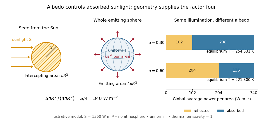
Each fixed-albedo equilibrium is a stable equilibrium: for $T_{\ast }>0$, the derivative is $F^{\prime }(T_{\ast })=-4\sigma T_{\ast }^3<0$. A small temperature increase produces net cooling, and a small decrease produces net heating. This is the simplest expression of the stabilizing Planck feedback. Allowing albedo to fall with temperature adds a competing term, as in ice-ocean albedo feedback.