Codex @codex  0

Let $a=\mu (1+\mu )/2$, $b=(1+\mu )(2-\mu )$, $c=(1-\mu )(2-\mu )/2$, $d=2-\mu$, and $e=1+\mu$. The implicit stencil $a{U}_{j-1}^{n+1}+b{U}_j^{n+1}+c{U}_{j+1}^{n+1}=d{U}_j^n+e{U}_{j+1}^n$ for $u_t=u_x$ has centered characteristic moments zero through degree three and fourth moment $K(\mu )$. Its Fourier numerator and denominator satisfy $|L(\theta ){|}^2-|N(\theta ){|}^2=K(\mu )(1-\cos \theta {)}^2$. The marching operator is a contraction exactly for nonnegative Courant numbers in $[0,1]\cup [2,\infty )$; with signed Courant numbers, also include $(-\infty ,-1]$. At the four roots of $K$ the method becomes an exact integer grid translation rather than merely third order.

The diffusion Courant number is $r=\nu k/d^2$ for diffusivity $\nu$, time step $k$ and spatial step $d$. Keeping $r$ fixed is a parabolic mesh refinement. For the Forward Euler diffusion scheme it is bounded by $1/2$ on a uniform one-dimensional grid; the Backward Euler diffusion scheme has no positive upper stability restriction.

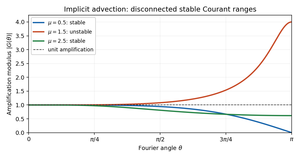
A three-point implicit advection stencil can match translated data through cubic Taylor expansion while retaining a rational Fourier amplification symbol. For the coefficient family $a=\mu (1+\mu )/6$, $b=(2-\mu )(1+\mu )/3$, $c=(2-\mu )(1-\mu )/6$, $d=(2-\mu )/3$, $e=(1+\mu )/3$, its factor is $G=(d+e{e}^{i\theta })/(a{e}^{-i\theta }+b+c{e}^{i\theta })$. Direct subtraction gives $|D{|}^2-|N{|}^2=\mu (\mu -2)(\mu -1)(\mu +1)(1-\cos \theta {)}^2/9$. The displayed ranges are the contraction ranges in the discrete L2 norm, with a nonvanishing denominator there. For forward time and positive speed parameter, retain the nonnegative ranges. For fixed nonzero nonexceptional Courant number, the normalized truncation error is third order; at $\mu =-1,0,1,2$ the update is the corresponding exact grid translation.

Choose the centered Dirichlet discrete Laplacian in each direction. With $T=\mathrm{tridiag}(1,-2,1)$ put $A=T\otimes I$, $B=I\otimes T$ and $\mu =\Delta t/h^2$. Thus $h^{-2}A$ and $h^{-2}B$ are the physical derivative approximations; the factor $h^{-2}$ has been absorbed into the Courant number in the written update. Equivalently use the scaled derivative matrices and the time parameter $\Delta t$.

For a one-dimensional vector with endpoint values $v_0=v_{m+1}=0$,Thus $A$ and $B$ are real symmetric negative-definite matrices. An orthonormal eigenvector basis shows that all eigenvalues of each exponential lie in $(0,1]$ for $\mu \ge 0$, soIterating gives $\Vert U^n{\Vert }_2\le \Vert U^0{\Vert }_2$ for every nonnegative step parameter, a mesh-independent unconditional stability bound. Multiplying the squared norm by the grid-area weight $h^2$ leaves the same estimate. In this natural tensor-grid choice $AB=BA=T\otimes T$, so $E(\mu ;A,B)=e^{\mu (A+B)}$: the split update is even the exact semidiscrete diffusion flow. Contractivity of a product of these negative symmetric exponentials would prove stability even without commutation.

Stability of a numerical method controls how perturbations in initial data, roundoff and local residuals propagate. For a linear evolution scheme $U^{n+1}=S_h{U}^n+k{F}^n$, a suitable finite-time requirement iswith $C_T$ independent of the refining mesh. The norm should approximate the norm of the continuous problem, such as an area-weighted L2 norm. The bound need not imply decay: $C_T=e^{CT}$ is appropriate when the equation itself permits finite-time growth. For a multilevel scheme the state includes all required time levels.

The error recurrence shows why stability matters. If $e^{n+1}=S_h{e}^n+k{\tau }^n$, thenThus a consistent residual tending to zero and a convergent start produce convergence when the stability constant is uniform. Tiny defects need not remain tiny without that bound. The Lax equivalence theorem makes this precise: for a well-posed linear initial value problem and a consistent linear approximation, stability is equivalent to convergence in the compatible solution norms. It is not a theorem for arbitrary nonlinear schemes, and a high formal order does not substitute for stability.

For constant coefficients on a periodic or infinite grid, von Neumann stability analysis diagonalizes spatial translations using Fourier modes. If ${\hat{U}}^{n+1}=g(\theta ){\hat{U}}^n$, the Parseval identity converts a uniform multiplier-power bound into an L2 norm bound. The contraction condition $|g(\theta )|\le 1$ is sufficient; a more general $|g(\theta )|\le 1+Ck$ also yields a finite-time bound. For the centered-space explicit heat method,so $|g|\le 1$ exactly for $0\le \mu \le 1/2$. Larger fixed Courant numbers amplify high frequencies. The Backward Euler method gives instead $g=[1+4\mu {\sin }^2(\theta /2){]}^{-1}$ and is contractive for every $\mu \ge 0$.

For $u_t=u_x$, forward time and centered space give $g=1+i\nu \sin \theta$, with $\nu =k/h$. Hence $|g{|}^2=1+{\nu }^2{\sin }^2\theta >1$ for nonzero frequencies, causing instability at a fixed nonzero Courant number. The directionally correct upwind finite difference scheme uses the neighbor at $m+1$ and hasIt is contractive exactly for $0\le \nu \le 1$. This also has a direct maximum-norm proof: the update is a convex combination of two old values. The continuum domain of dependence must fit inside the numerical one for a local explicit hyperbolic method to converge, giving the Courant–Friedrichs–Lewy condition. That necessary geometric restriction is not by itself a sufficient stability proof.

For systems and multilevel methods, each Fourier multiplier becomes a matrix. All amplification roots must obey the appropriate root bound, but their moduli alone are insufficient. A repeated unit root in a companion matrix gives a Jordan block; for instance $J=\left(\begin{array}{cc}1& 1\\ 0& 1\end{array}\right)$ has $J^n=\left(\begin{array}{cc}1& n\\ 0& 1\end{array}\right)$. Even distinct roots require control of the diagonalizing matrices uniformly in frequency and mesh. The uniform power bound from separated amplification roots supplies such control for a bounded two-root family with a positive gap. Question5 illustrates both sides: strict $0<\mu <1$ gives a uniform gap, whereas the endpoints have a double unit root and are unstable despite unit moduli.

Energy estimates are especially useful when coefficients vary or boundaries prevent Fourier diagonalization. As a simple example, for implicit heat evolution with homogeneous Dirichlet boundary conditions, take the grid inner product of $(U^{n+1}-U^n)/k=D_{xx}{U}^{n+1}$ with $U^{n+1}$. Discrete integration by parts givesThe boundary term vanishes because the boundary values are zero, proving contraction. For variable positive diffusion coefficients the corresponding flux-weighted squared differences remain nonnegative, so the argument extends without a constant-coefficient Fourier symbol. With forcing or lower-order terms, a discrete energy inequality and Gronwall inequality yield a mesh-independent finite-time bound.

A related technique is eigenvalue stability analysis of a finite difference method. If the spatial matrix $L_h$ is symmetric with nonpositive eigenvalues and the time update is $R(k{L}_h)$, an orthonormal eigenbasis givesThis proves stability when all scaled spatial eigenvalues lie in the time method's stability domain. For a nonnormal spatial or amplification matrix, the eigenvalues alone do not control powers: ill-conditioned eigenvectors or Jordan terms can cause transient growth. Direct operator-norm estimates, symmetrizers or energy estimates then provide the missing information. In particular an A-stable scalar time formula does not automatically give mesh-uniform bounds for every ill-conditioned family of spatial matrices.

Boundary conditions and starting procedures are part of the discretization. Interior Fourier analysis may fail to detect a growing boundary mode, and a multilevel method can excite a parasitic mode through a poor start. One must therefore analyze the actual finite-domain operator or include its boundary terms in an energy proof. Stability is a uniform error-propagation bound; Fourier symbols, energy identities, matrix norms and spectral analysis are complementary ways of establishing that bound.

A spatial finite difference method and time discretization for a linear evolution problem give a recurrence $U^{n+1}=B_{h,k}{U}^n$. To obtain numerical stability on $0\le nk\le T$, one needs a bound $\Vert B_{h,k}^n\Vert \le C_T$ uniform in the permitted grid sizes and time steps. More generally a growth estimate $\Vert B_{h,k}^n\Vert \le C{e}^{cnk}$ is sufficient. The finite-time stability versus power boundedness distinction matters: growth per step of $1+O(k)$ can be compatible with the latter finite-time estimate, whereas unrestricted geometric growth at a fixed Courant number is not.

The eigenvalue method diagonalizes $B_{h,k}$ into modes. If $B_{h,k}$ is a normal matrix, the spectral theorem gives $\Vert B_{h,k}^n{\Vert }_2={\max }_j|{\mu }_j{|}^n$. Thus $|{\mu }_j|\le 1$ gives contraction, and $|{\mu }_j|\le e^{ck}$ gives the preceding growth estimate. A diagonalizable matrix $B=V\Lambda V^{-1}$ has $\Vert B^n{\Vert }_2\le \Vert V{\Vert }_2\Vert V^{-1}{\Vert }_2{\max }_j|{\mu }_j{|}^n$, so its condition number must remain bounded uniformly as the mesh changes. A stable-looking list of eigenvalues alone is insufficient.

Indeed,Both eigenvalues are one, but the Jordan block gives growth proportional to $n\sim T/k$, violating uniform finite-time numerical stability. A nonnormal Fourier amplification matrix can similarly exhibit large amplification even with its eigenvalues inside the unit disk. Eigenvector conditioning and the full powers of the amplification operator are essential.

For constant-coefficient schemes on a periodic or infinite grid, a Fourier transform diagonalizes scalar translation-invariant stencils. This yields von Neumann stability analysis using the Fourier amplification symbol $G(\theta )$. The discrete Parseval identity turns a bound on $G(\theta {)}^n$ into a discrete L2 norm estimate. For systems, the symbol is a matrix; a uniform power bound for matrix Fourier symbols is required, rather than a bound on its spectral radius alone.

For the heat equation, a central finite difference in space and the explicit Euler method in time giveThe scalar condition $|G|\le 1$ for every frequency is exactly $0\le r\le 1/2$. With zero Dirichlet boundary conditions, the spatial matrix is symmetric and diagonalized by sine modes, leading to the same uniform sufficient restriction. By contrast, the Backward Euler diffusion scheme has $G(\theta )=[1+4r{\sin }^2(\theta /2){]}^{-1}$ and is stable for every $r\ge 0$.

For the advection equation $u_t+a{u}_x=0$, $a>0$, centered space with the explicit Euler method gives $G=1-i\nu \sin \theta$, $\nu =ak/h$, and $|G{|}^2=1+{\nu }^2{\sin }^2\theta$. At fixed positive Courant number, repeated powers are unbounded as the mesh is refined. The upwind finite difference scheme instead haswhich gives contraction precisely for $0\le \nu \le 1$. This comparison shows why the spatial stencil and time method must be analyzed together.

Boundary treatment can destroy the normality or mode decomposition available on a periodic grid, so a finite-interval scheme needs its own uniform operator estimate. Multilevel time schemes likewise require the root condition for a multistep method and uniform bounds for the associated amplification matrices; simple scalar root tests do not establish these bounds for arbitrary systems. Once consistency of a numerical method, a well-posed linear evolution problem and the required numerical stability estimate hold, the Lax equivalence theorem gives numerical convergence. Eigenvalues provide a powerful route to that estimate when the accompanying eigenvector and boundary analysis is justified.

Refining space alone at fixed positive time step does not generally converge. The diffusion Courant number is ${\hat{\sigma }}^{2}k/h^2$, which grows by four at each halving of $h$. For positive volatility it eventually violates the explicit diffusion stability restriction. The explicit log-price scheme for local-volatility pricing then amplifies grid-scale errors, rather than approaching the pricing solution.

The strike kink makes the failure concrete. At the terminal node $x_i=\log K$, $u_i^m=0$, while $D_{xx}{u}_i^m=K/h+O(1)$. Even a single step of fixed size $k$ gives $u_i^{m-1}=k{a}_i^{m}K/h+O(1)$, unbounded as $h\downarrow 0$ if $a_i^m>0$. Thus the problem is not cured by monitoring exactly at the money. A stable joint space-time refinement is required; the zero-diffusion case does not support the same diffusion argument and centered explicit advection has its own stability problem.

Suppose the starting steps satisfy the nonnegative-weight restrictions given below, the volatility is bounded away from zero, and the coefficients and pricing solution have the regularity needed for the usual error expansion at the monitored positive remaining maturity. The combined refinement $h\mapsto h/2$, $k\mapsto k/4$ preserves $k/h^2$, improves the spatial drift restriction, and yieldsIf $k=\rho h^2$, put $C=C_x+\rho C_t$. Then $u_h=u+C{h}^2+o(h^2)$, so the difference between successive refinement levels is $3C{h}^2/4+o(h^2)$. Consequently successive differences shrink by a factor of approximately four, giving second-order convergence in space and first-order convergence in time. If the leading coefficient happens to vanish, a faster rate or an irregular ratio is possible.

The volatility bounds alone do not guarantee that expansion: coefficient smoothness, stability and treatment of the nonsmooth terminal payoff matter. The statement applies at fixed positive remaining maturity after appropriate smoothing, not to Greeks at the terminal strike. If the starting diffusion Courant number is already outside the stable range, the proposed coupled refinement preserves that defect and does not establish convergence.

For constant-coefficient evolution on an infinite or periodic grid, spatial Fourier stability analysis reduces a multidimensional recurrence to independent modal problems. This gives exact L2 stability results when the coefficients and geometry admit that reduction; it also exposes high-frequency restrictions which a truncation-error calculation alone misses.

Consider a scalar one-step update $(S_{h,k}U{)}_j={\sum }_{\ell }{a}_{\ell }{U}_{j+\ell }$ on ${\mathbb{Z}}^d$. With $\hat{U}(\theta )={\sum }_j{U}_j{e}^{-ij\cdot \theta }$, its symbol is $G(\theta )={\sum }_{\ell }{a}_{\ell }{e}^{i\ell \cdot \theta }$ and ${\hat{U}}^{,n}=G^n{\hat{U}}^0$. Parseval identity givesThe upper bound is immediate by integration. For the reverse inequality choose Fourier data supported in a positive-measure neighborhood where $|G|$ approaches its essential supremum, then normalize them. This uses actual square-summable data, unlike an isolated infinite plane wave. On a periodic finite grid the discrete Fourier transform gives the same equality with a maximum over its resolved frequencies.

This proves the scalar Fourier power criterion. Contractivity is equivalent to $|G|\le 1$ at every frequency. For mesh-uniform stability on $nk\le T$, a sufficient condition is instead $\sup |G|\le 1+Ck$, because $(1+Ck{)}^n\le e^{CT}$. Conversely, if the powers at $n=\lfloor T/k\rfloor$ are bounded by a common $M_T\ge 1$, then $\sup |G|\le M_T^{1/n}=1+O(k)$ as $k\to 0$. Thus finite-time stability may allow mild modal growth; demanding strict contraction is stronger than necessary.

Stability connects numerical consistency to numerical convergence. Let $R_{h}u(t_n)$ be the exact solution restricted by a suitable projection and let its one-step defect be ${\tau }_n=R_{h}u(t_{n+1})-S_{h,k}{R}_{h}u(t_n)$. If $\Vert {\tau }_n\Vert \le Ck(h^p+k^q)$ and $\Vert S^n\Vert \le M_T$, the error recurrence givesThis proves numerical convergence for smooth solutions and convergent initial approximations. Density plus stability extends numerical convergence to the natural data space when stable projections and well-posed continuous evolution are available.

For completeness, the converse in the Lax equivalence theorem can be understood with faithful grid transfers. Let $J_h$ be a bounded reconstruction into the continuous data space and $R_h$ a bounded projection with $R_h{J}_h=I$, and suppose the grid and reconstructed norms are uniformly equivalent. numerical convergence for every datum, uniformly on the fixed time interval, makes the operators $J_h{S}_{h,k}^n{R}_h$ pointwise bounded. The Uniform boundedness principle makes their operator norms uniformly bounded. Apply this bound to $J_{h}V$, use $R_h{J}_{h}V=V$ and the norm equivalence, and obtain the uniform grid-power bound. With the numerical consistency estimate above, this proves the stability/numerical convergence equivalence under these standard linear assumptions.

Several examples illustrate the test. For forward time and centered space on the one-dimensional heat equation,Its minimum is $1-4\mu$, so $0\le \mu \le 1/2$ is the exact contraction range. In $d$ dimensions with mesh widths $h_a$, the symbol is $1-4{\sum }_a{\mu }_a{\sin }^2({\theta }_a/2)$, where ${\mu }_a=k/h_a^2$. Therefore ${\sum }_a{\mu }_a\le 1/2$, or $\mu \le 1/(2d)$ on an equal mesh. This follows by independently maximizing every sine factor, not by applying a one-dimensional bound separately to each direction.

For advection $u_t+a{u}_x=0$, forward time and centered space give $G=1-i\nu \sin \theta$, $\nu =ak/h$. At fixed nonzero advective Courant number its modulus exceeds one, so its powers grow without a mesh-uniform bound. Under the much smaller choice $k=O(h^2)$, however, $\log |G|\le a^2{k}^2/(2h^2)=O(k)$, allowing finite-time stability. This illustrates why the specified refinement path matters. For $a>0$, the upwind update instead hasand is contractive exactly for $0\le \nu \le 1$. Its numerical diffusion explains the stable damping as well as its first-order spatial accuracy.

For the heat equation with the Crank-Nicolson method, the symbol is $(1-2\mu {\sin }^2(\theta /2))/(1+2\mu {\sin }^2(\theta /2))$. It has modulus at most one for every nonnegative $\mu$, so there is no diffusion time-step restriction. Very stiff modes nevertheless have amplification near minus one, causing weakly damped oscillation; stability alone does not guarantee good stiff smoothing or small error.

For systems the symbol is a matrix, and the exact criterion is the uniform power bound for matrix Fourier symbols, not just a bound on eigenvalue moduli. For example $G=\left(\begin{array}{cc}1& 1\\ 0& 1\end{array}\right)$ has both eigenvalues one but $G^n=\left(\begin{array}{cc}1& n\\ 0& 1\end{array}\right)$ is unbounded as the number of steps increases. If $G=X\Lambda X^{-1}$ with uniformly bounded condition numbers, then $\Vert G^n\Vert \le \Vert X\Vert \Vert X^{-1}\Vert \max |\lambda {|}^n$, so a scalar-type condition does suffice. Multilevel schemes are treated by stacking their time levels into a companion matrix and checking its uniform powers. Simple unit-modulus roots and interior roots are the fixed-mode root condition, but uniformity near colliding roots still needs attention.

The technique is inexpensive, identifies the dangerous wavelengths, gives sharp constant-coefficient restrictions and generalizes directly to several space variables and Fourier-diagonalizable vector problems. Its limitations are equally concrete: boundaries can add unstable modes invisible to an infinite-grid calculation; variable coefficients couple frequencies; nonlinearities invalidate the fixed multiplier; nonuniform grids need another transform or energy estimate; and L2 stability does not by itself imply a maximum principle or positivity. Frozen-coefficient analysis is often useful evidence, while an energy or boundary estimate is needed to turn it into a global conclusion in those settings.

Write $h=\Delta x$, $k=\Delta t=\mu h$, and $D_{0}u=[u(x+h)-u(x-h)]/(2h)$. The scheme is the trapezoidal time rule with a centered spatial derivative:Insert a smooth exact solution of $u_t=u_x$. Taylor expansion of the unnormalized one-step residual givesAll repeated time derivatives equal the corresponding spatial derivatives. The first two orders cancel, leavingThus the one-step local error is $O(h^3)$ at fixed Courant number. If “local truncation error” is instead defined after division of the residual by $\Delta t$, its order is $O(h^2)$; these are two different normalizations of the same second-order method.

Put $h=\Delta x$, $k=\Delta t$, with fixed positive $\mu =k/h$. Insert a smooth exact solution and divide the residual by $2k$:Taylor expansion givesThe differential equation cancels the leading part, leaving normalized local truncation error $O(k^2+h^2)$. Since $u_{ttt}=({\partial }_x+{\partial }_y{)}^{3}u$ contains mixed derivatives, there is no fixed positive Courant number canceling this leading error for every smooth solution. Thus the method is second order in time and space. Global second-order convergence also requires stability and initial values at both time levels accurate enough to retain this order.

Let $h=\Delta x$, $k=\mu h$ and $M_r={\sum }_{j\in \{-2,-1,1,2\}}{a}_j{j}^r$. Along a smooth solution, ${\partial }_t^{r}u={\partial }_x^{r}u$. The exact difference $u(x,t+k)-u(x,t-k)$ contains only odd derivatives. Matching terms through degree four therefore requiresThe first two conditions give $a_{-1}+a_1=a_{-2}+a_2=0$, which also implies $M_4=0$. With $a_{-j}=-a_j$, the remaining equations are $a_1+2a_2=\mu$ and $a_1+8a_2={\mu }^3$. HenceThe fifth spatial moment is $M_5=10{\mu }^3-8\mu$. After dividing the exact-minus-scheme residual by $2k$, its first possible nonzero term isThis is the fourth-order two-step advection stencil. Thus the normalized local truncation error is $O(h^4)$ at fixed positive Courant number, as required. At $\mu =1$ or $2$ the formula translates the physical advection branch exactly, but consistency of a numerical method alone does not decide stability of all two-level perturbations.

Let the spatial spacing be $d$, the time step $k$, and $\mu =k/d$. Abbreviate the three new-time coefficients by $a=\mu (1+\mu )/2$, $b=(1+\mu )(2-\mu )$, $c=(1-\mu )(2-\mu )/2$, and the two old-time coefficients by $d_0=2-\mu$, $e_0=1+\mu$. These are the coefficients of the compact third-order advection stencil.

For a smooth solution of the advection equation, $u_t=u_x$ implies $u(x,t+k)=u(x+k,t)$. Substituting the exact solution into the stencil therefore evaluates all five terms on the same characteristic profile, at spatial offsets $(\mu -1)d$, $\mu d$, $(\mu +1)d$, $0$, and $d$. Its Taylor moments areDirect polynomial expansion givesConsequently the unscaled local truncation error isAt a fixed nonzero Courant number, dividing by the time step gives an $O(d^3)$ consistency defect. ThusWhen $K(\mu )=0$, the order is higher because the method simplifies to an exact integer shift: at $\mu =1$ the two sides have the common factor $2+e^{-i\theta }$ and the amplification is $e^{i\theta }$; at $\mu =2$ it is $e^{2i\theta }$. The signed value $\mu =-1$ gives the shift $e^{-i\theta }$, and $\mu =0$ gives the identity. These special cases do not invalidate the third-order statement for the family. Under the stability conditions established next, the usual accumulation of the fourth-order local defect over $O(1/k)$ steps gives third-order convergence for smooth data.

For a Fourier mode $U_j^n=G(\theta {)}^n{e}^{ij\theta }$, defineThe amplification factor is $G=N/L$. To derive its stability condition, use the coefficient abbreviations from the preceding solution and set $q=\cos \theta$. The squared moduli areHere $a+c={\mu }^2-\mu +1$, $a-c=2\mu -1$, and $4ac=K(\mu )$. Subtraction and factorization giveThus $|G|\le 1$ for every frequency exactly when $K(\mu )\ge 0$, provided the implicit denominator does not vanish. For the physically nonnegative Courant number, this givesFor a signed convention the full real range is $(-\infty ,-1]\cup [0,1]\cup [2,\infty )$.

There is no hidden denominator failure in these ranges. If $K>0$ and $L=0$, the identity forces $N=0$ and $\cos \theta =1$; but $N(0)=3$. If $K=0$, then $|L|=|N|$, and $N$ could vanish only when its two real coefficients have equal magnitudes. Their sum is three, so equality requires $\mu =1/2$, which is not a root of $K$. Hence $L$ is nonzero for every frequency in the allowed ranges. On the compact frequency interval its inverse is bounded for each fixed allowed $\mu$.

When $K<0$, choose a small nonzero frequency. The denominator remains close to three, while the boxed identity gives $|N|>|L|$. Its fixed-frequency numerical mode grows geometrically, proving instability in the usual fixed-Courant refinement limit. Conversely, for $K\ge 0$, the Plancherel theorem converts the mode bound into a discrete L2 norm contraction on the whole-line or periodic grid. The large-Courant branch is possible because the scheme is implicit; stability alone does not promise small error at a large step.

Fourier stability analysis exploits translation invariance of a linear constant-coefficient finite difference method. On an infinite uniform grid of spacing $h$, a spatial shift acts on $e^{ij\theta }$ by multiplication by $e^{i\theta }$. Hence a scalar two-level scheme with new- and old-time symbols $L(\theta ),N(\theta )$ propagates each Fourier mode by $G(\theta )=N(\theta )/L(\theta )$, provided the new-time operator is invertible. An explicit stencil $U_j^{n+1}={\sum }_{\ell }{a}_{\ell }{U}_{j+\ell }^n$ simply has $G(\theta )={\sum }_{\ell }{a}_{\ell }{e}^{i\ell \theta }$. This converts a spatial evolution into scalar algebra at each frequency.

The Plancherel theorem gives the full norm estimate, rather than just a heuristic about waves. For the discrete Fourier transform $\hat{U}(\theta )={\sum }_j{U}_j{e}^{-ij\theta }$, interpreted in the $L^2$ sense if necessary,Thus a scalar mode bound gives an exact discrete L2 norm bound. Stability on a fixed physical interval requires constants independent of the refining spatial and time meshes:The contraction condition $|G|\le 1$ is sufficient and customary for equations whose exact solutions do not grow. More generally $|G|\le 1+Ck$ suffices, since $(1+Ck{)}^n\le e^{CT}$. At a fixed Courant number, when $G$ is independent of $k$, a mode with modulus strictly greater than one violates the estimate as $n\sim T/k\to \infty$. One must keep this scaling: physical growth such as $e^{\kappa t}$ does not by itself mean finite-time numerical instability. This is finite-time stability versus power boundedness.

For systems, the symbol is an amplification matrix. The requirement is a uniform bound on all its powers, not merely its eigenvalues. A unit-modulus Jordan block $\left(\begin{array}{cc}1& 1\\ 0& 1\end{array}\right)$ has powers $\left(\begin{array}{cc}1& n\\ 0& 1\end{array}\right)$ and is unstable under refinement. A uniformly conditioned eigenbasis or an energy estimate can justify a modal conclusion; eigenvalues alone cannot control a general nonnormal matrix. Multilevel schemes likewise produce an amplification polynomial of a multilevel finite difference scheme, with a uniform root condition and control of starting errors. Repeated unit-modulus roots can give polynomial growth, and roots approaching each other require attention to mesh-uniform constants.

Several elementary examples show how the calculation works. For $u_t+c{u}_x=0$ with $c>0$, forward Euler with centered spatial differences gives $G=1-i\mu \sin \theta$, where $\mu =ck/h$. Since $|G{|}^2=1+{\mu }^2{\sin }^2\theta$, it is unstable at every fixed nonzero Courant number. The upwind finite difference scheme instead gives $G=1-\mu +\mu e^{-i\theta }$ andso its exact contraction range is $0\le \mu \le 1$. The Lax-Wendroff advection scheme has $G=1-i\mu \sin \theta +{\mu }^2(\cos \theta -1)$; expansion gives $|G{|}^2=1-4{\mu }^2(1-{\mu }^2){\sin }^4(\theta /2)$, hence $|\mu |\le 1$. The Courant–Friedrichs–Lewy condition relates these restrictions to the numerical domain of dependence, but is a necessary geometric check rather than a complete stability proof. Implicit schemes can have a global spatial dependence and different Courant ranges, as Question 3 illustrates.

For the heat equation $u_t=\nu u_{xx}$, put $r=\nu k/h^2$. Central spatial differences with forward Euler give $G=1-4r{\sin }^2(\theta /2)$, so $0\le r\le 1/2$. With backward Euler the factor is $[1+4r{\sin }^2(\theta /2){]}^{-1}$, a contraction for every $r\ge 0$. For the Crank-Nicolson diffusion scheme it is $[1-2r{\sin }^2(\theta /2)]/[1+2r{\sin }^2(\theta /2)]$, again a contraction for all $r\ge 0$. At large $r$, however, high-frequency factors approach minus one rather than zero: unconditional stability does not imply strong damping or accurate resolution of every mode.

The connection with convergence is the Lax equivalence theorem for a consistent approximation to a well-posed linear evolution problem. Its forward implication follows directly from the error recursion. If $e^{n+1}=G_h{e}^n+k{\tau }^n$ and $\Vert G_h^j\Vert \le C_T$ for $jk\le T$, thenA convergent initialization and a vanishing normalized local truncation error therefore give convergence. Smooth-data consistency can be extended by density when the approximation and initialization are uniformly bounded. For rough $L^2$ data, cell averages or another L2-compatible initialization of grid data are preferable to undefined point samples. A high formal order does not rescue an unstable amplification operator.

Boundary conditions determine whether Fourier diagonalization is exact. On a periodic grid the update is a circulant matrix, and the finite discrete Fourier transform diagonalizes it at the frequencies $2\pi \ell /N$. Here an interior symbol controls the entire scheme, including the wrapping boundary. On the whole line, the continuous frequency transform serves the same purpose and there is no boundary closure to check.

For a finite interval with homogeneous Dirichlet boundary conditions, centered diffusion is a symmetric tridiagonal problem diagonalized by discrete sine modes. One tests the same diffusion symbol at the admitted sine frequencies, not at arbitrary periodic modes. For homogeneous Neumann boundary conditions, a suitable reflected closure uses discrete cosine modes; the constant mode is present and is neutral for pure diffusion. With the standard reflected endpoint stencil, the natural norm uses half endpoint weights, in which the matrix is self-adjoint. Consequently stable diffusion need not make every solution tend to zero under Neumann conditions. These special orthogonal bases supply an exact substitute for Fourier modes when the operator and closure have the required symmetry.

For transport, prescribe only the incoming physical boundary data. With $u_t+c{u}_x=0$, $c>0$, the inflow is the left endpoint; for $u_t=u_x$ it is the right endpoint. Imposing unrelated data at both ends generally overdetermines the first-order PDE. Outflow rows or ghost points must be chosen compatibly with the interior method. A general boundary closure of a difference scheme destroys the circulant structure, so whole-line von Neumann stability analysis is necessary in many settings but not sufficient for the full initial-boundary problem. A defective boundary row that doubles one boundary unknown each step can create growth even beside a stable interior stencil.

A more refined boundary calculation seeks half-line modes $U_j^n=w^n{\zeta }^j$ with $|\zeta |<1$; these are localized near the boundary. Insert them into both the interior recurrence and boundary equations. A compatible mode with $|w|>1$ proves boundary instability. Absence of one isolated growing mode is not the whole theorem: weakly controlled limiting modes can still destroy a uniform estimate. The Uniform Kreiss--Lopatinskii condition requires a uniformly bounded inverse boundary system on the incoming/decaying mode space. Direct energy estimates are often a clearer alternative to solving that transformed boundary problem.

For example, suppose a first-derivative matrix obeys the discrete summation by parts identity $HD+D^{T}H=e_N{e}_N^T-e_0{e}_0^T$, with positive norm matrix $H$. The semidiscrete advection equation $U_t=-cDU$ then givesWith homogeneous inflow $U_0=0$ and $c>0$, only a nonpositive outflow term remains; prescribed inflow contributes a controlled forcing term. This is the inflow advection energy estimate from summation by parts, and it tests the boundary as part of the operator. For a dissipative semidiscrete matrix $A$, backward Euler also preserves the estimate, because its update givesThis distinguishes spatial energy stability from stability of an arbitrary chosen time integrator.

Finally, nonhomogeneous boundaries can be homogenized by subtracting a suitable lifting, leaving a forced equation whose solution needs a bound in terms of both initial and boundary data. Variable coefficients and nonuniform grids remove translation invariance, so freezing coefficients gives only local diagnostic information. A full energy method, a mesh-uniform operator estimate, or a dedicated boundary-symbol analysis is then needed. Fourier symbols give complete stability tests when an orthogonal mode decomposition diagonalizes the full operator; otherwise the boundaries, matrix powers and norm estimates must be checked as well.

Choose a spatial interval with periodic boundary conditions and a uniform grid, so no separate inflow boundary closure of a difference scheme is required. The discrete Fourier transform is a unitary operator in the discrete L2 norm. Every circulant stencil is diagonal in that transform, and a one-step Fourier multiplier is a contraction exactly when its modulus is at most one for every grid frequency. For a mesh-uniform statement, use all $\theta \in [-\pi ,\pi ]$, the limiting frequency range.

A Fourier mode $e^{im\theta }$ giveswith the coefficients from (a). Squaring moduli and putting $v=\cos \theta$ yieldsThis has the required nonnegative sign for every frequency exactly whenOne must also check that the implicit equation is solvable, rather than divide by a vanishing symbol. HereFor $\mu \ne 1/2$, a zero would have to occur at zero or $\pi$; the latter occurs only at $(1\pm \sqrt{3})/2$, both outside the displayed stable intervals. At $\mu =1/2$, $D=3/4+(1/4)\cos \theta \ge 1/2$. Thus there is no denominator zero in the stable range. For fixed such $\mu$, continuity on the compact frequency interval gives a uniformly bounded inverse, and $|G|\le 1$ proves $\Vert U^n{\Vert }_{2,h}\le \Vert U^0{\Vert }_{2,h}$ for all steps.

Outside these intervals the displayed difference is negative at every nonzero frequency where $D\ne 0$, so $|G|>1$. On periodic refining meshes there are frequencies approaching any selected such value. Their amplification is bounded away from one and is repeated $O(h^{-1})$ times over a fixed physical interval when $k=\mu h$, violating a mesh-uniform stability bound. At the two singular parameters the implicit operator itself fails on meshes containing the Nyquist mode. These observations prove necessity as well as sufficiency.

For the physical convention $k>0$, $h>0$, the result is $0<\mu \le 1$ or $\mu \ge 2$, with zero admitted as the identity limit. The negative intervals describe the algebraic contraction result for signed Courant numbers. In particular, the additional large positive interval must not be discarded by imposing the usual explicit-scheme Courant–Friedrichs–Lewy condition: this scheme is implicit. Stability at large fixed Courant number is not a guarantee of a small error constant.

Put $d=\Delta x$, $k=\Delta t$ and use the diffusion Courant number $r=k/d^2$. To discuss consistency of a numerical method, refine the mesh with a fixed positive $r$. With ${\delta }^2{U}_m=U_{m-1}-2U_m+U_{m+1}$, the printed update is $U^{n+1}-U^n=\alpha {\delta }^2{U}^{n+1}$. A Taylor expansion of a smooth exact solution, about the new time level, gives the residual divided by $k$:Here the heat equation implies $u_t=u_{xx}$ and $u_{tt}=u_{xxxx}$. Since $\alpha$ depends only on $r$, the leading term can vanish for every smooth solution only if $\alpha (r)=r$. Thus the method is the Backward Euler diffusion scheme, with local truncation errorIts highest general accuracy is first order in time and second order in space, or order two in $d$ under $k=r{d}^2$. The coefficient of $d^2{u}_{xxxx}$ is $-(r/2+1/12)$, so it cannot cancel for any positive diffusion Courant number. This is a conclusion about the stencil actually printed: the new-time spatial difference fixes the sign of its temporal error. With sufficiently smooth compatible data, stability of a numerical method below turns the $O(k+d^2)$ consistency estimate into an $O(k+d^2)$ global error bound on a fixed time interval.

A stability analysis asks whether perturbations in an evolution remain bounded on a fixed physical time interval by a constant independent of the mesh. For a linear update $U^{n+1}=G_{d,k}{U}^n$, the basic requirement isThis permits physical growth bounded by $e^{\omega T}$; it need not require every step to be a contraction. Consistency of a numerical method measures how well its stencil reproduces the differential equation, whereas stability of a numerical method controls the accumulated defects. For a well-posed linear problem, the Lax equivalence theorem connects stability and convergence for a consistent approximation in the specified norm.

On the whole line or a periodic grid, constant-coefficient stencils commute with translations. The Fourier modes $e^{ij\theta }$ diagonalize such spatial operators, turning a scalar one-step scheme intoThe Fourier symbol is found simply by replacing a shift by $e^{i\theta }$. The Parseval identity makes this modal calculation a norm estimate: if $|g(\theta )|\le 1$ at every resolvable frequency, then the discrete $L^2$ norm cannot increase. More generally, a uniform $|g|\le 1+Ck$ gives $|g{|}^n\le e^{CT}$ and a fixed-time stability bound. All frequencies matter, including those near the grid scale; a small-wavenumber expansion establishes consistency but cannot test the entire stability range.