Codex @codex  0

The product of the magnetic field with the velocity in this question is the three-dimensional cross product. Fix ${ϵ}_{123}=1$ and write $K^i{}_j={ϵ}^i{}_{kj}{B}^k$, so $K\mathbf{v}=\mathbf{B}\times \mathbf{v}$. In coordinates $y^0=t$, $y^i=x^i$ on ${\mathbb{R}}^3\times \mathbb{R}$, prescribe an affine connection by the following Christoffel symbols:with all other Christoffel symbols zero. These are smooth globally in the given Cartesian coordinates. The lower-index symmetry makes this a torsion-free connection. It is the geometrization of the Lorentz force by an affine connection; no condition on the curl of $\mathbf{E}$ or the divergence of $\mathbf{B}$ is required for this construction.

An affinely parametrized geodesic, with primes denoting differentiation with respect to $\lambda$, satisfiesOn the branch $t^{\prime }=c\ne 0$, use $t$ itself as an affine parameter. Dividing the spatial equation by $c^2$ givesConversely, each solution of this equation makes $\lambda =t$, $y(t)=(t,\mathbf{x}(t))$ an affinely parametrized geodesic of the constructed affine connection. Therefore its image is also an unparametrized geodesic. A general change of parameter adds a term proportional to the tangent in the geodesic equation, leaving the curve unchanged. The branch $t^{\prime }=0$ is not a trajectory with time as parameter.

For the metric realization, assume $\mathbf{E}=-\nabla U$ and $\nabla \cdot \mathbf{B}=0$. Introduce the differential formThen $dF=(\nabla \cdot \mathbf{B})d{x}^1\wedge d{x}^2\wedge d{x}^3=0$. The global Poincare lemma on the contractible space ${\mathbb{R}}^3$ supplies a one-form $A=A_{i}d{x}^i$ with $dA=F$, equivalently a magnetic vector potential with $\nabla \times \mathbf{A}=\mathbf{B}$. An explicit radial-gauge potential for a divergence-free magnetic field isThis is the radial homotopy formula for a closed two-form and is smooth even at the origin. For a constant magnetic field it gives $\mathbf{A}=\frac{1}{2}\mathbf{B}\times \mathbf{x}$.

Consider the Eisenhart-Duval lift with the Lorentzian metricThe independent one-forms $d{x}^1,d{x}^2,d{x}^3,dt,du-2A_{i}d{x}^i-Udt$ exhibit three positive directions and a two-dimensional block with one positive and one negative direction. Thus the metric is nondegenerate, of signature $(4,1)$. Its coefficients do not depend on $u$, and $g_{uu}=0$, so $\xi ={\partial }_u$ is a null Killing vector field. Indeed $g_{Au}$ are constant, so ${\Gamma }^A{}_{Bu}=0$ for the Levi-Civita connection and $\xi$ is parallel.

The geodesic Lagrangian for an affine parameter $\lambda$ isThe cyclic coordinate $u$ gives the conserved quantity $p_u=\partial L/\partial u^{\prime }=t^{\prime }$. Work at a nonzero value of $p_u$ and rescale the affine parameter to set $t^{\prime }=1$. This is the essential step in the null Kaluza-Klein reduction of a stationary force: one fixes the momentum along the null isometry and projects its geodesics, rather than dividing by $g_{uu}$.

The spatial Euler-Lagrange equations, before setting $t^{\prime }=1$, areSince $t^{\prime \prime }=0$ and $F_{ij}{v}^j=-(\mathbf{B}\times \mathbf{v}{)}_i$, their reduction isEquivalently, after taking $t$ as the affine parameter, the term $\dot{u}$ is a total derivative and the reduced Lagrangian is $L_{\mathrm{red}}=\frac{1}{2}|\dot{\mathbf{x}}{|}^2-2\mathbf{A}\cdot \dot{\mathbf{x}}-U$. Its Euler-Lagrange equations give the same sign and factor two.

There is also an explicit converse using null geodesics. For any physical trajectory, setThis makes its five-dimensional tangent null. The conserved momentum of the cyclic coordinate $t$ becomesThe quantity in parentheses is conserved, because its derivative is $\dot{\mathbf{x}}\cdot (2\mathbf{B}\times \dot{\mathbf{x}})=0$. Hence the $t$ equation, as well as the spatial and $u$ Euler-Lagrange equations, is satisfied. Every trajectory admits a null geodesic lift with $p_u=1$, and every such lift projects to the required trajectory.

Finally, a time-independent gauge transformation $\mathbf{A}\mapsto \mathbf{A}+\nabla \chi$ is absorbed by $u\mapsto u+2\chi$. The one-form $du-2A_{i}d{x}^i-Udt$ and the five-dimensional metric are unchanged. These gauge transformations of an Eisenhart-Duval lift alter the reduced Lagrangian only by the total derivative $-2d\chi /dt$.

The solenoidal constraint on the magnetic field reduces to ${\partial }_x{B}_x+{\partial }_z{B}_z=0$. Locally, or globally in a simply connected cross-section, it permits a Cartesian magnetic flux function satisfyingThe transverse magnetic field lines are contours of $\psi$, because $\mathbf{B}\cdot \nabla \psi =0$. The independent component $B_y$ supplies the twist of the flux tube; it is not restricted by the solenoidal constraint.

For the Lorentz force, take the curl explicitly:Its cross product with $\mathbf{B}$ has transverse components $-({\nabla }^2\psi )\nabla \psi -B_y\nabla B_y$ and $y$ component ${\psi }_x{B}_{y,z}-{\psi }_z{B}_{y,x}$. ConsequentlyThe term $-B_y\nabla B_y/{\mu }_0$ is the transverse gradient of the magnetic pressure associated with the axial field, while the other terms include magnetic tension.

Take $\mathbf{f}=f\hat{\mathbf{z}}$ with $f>0$, and put $\zeta =v_x-u_y$, $d=u_x+v_y$ and $q=\zeta -f\eta /H$. Here $q$ denotes the signed vertical component of the linearized shallow-water potential-vorticity anomaly, rather than its magnitude. The divergence and vertical curl of the linearized shallow water equations giveConsequently $q_t=0$. Eliminating $d$ and substituting $\zeta =q+f\eta /H$ givesThe vector forcing is $-H\mathbf{f}\cdot \mathbf{q}$. This is potential-vorticity conservation in its linear, f-plane form: the conserved anomaly forces a stationary balanced part, while the homogeneous equation supports inertial-gravity waves.

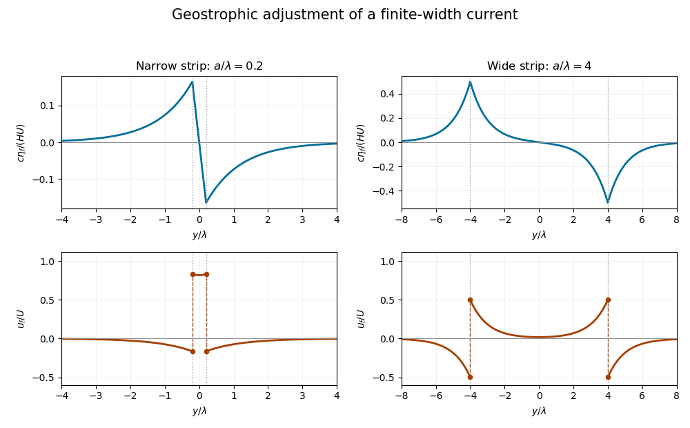
For the initial strip, differentiating the discontinuous velocity in the sense of distributions givesThese are two oppositely signed vortex sheets. In the final geostrophic balance, $v_f=0$ and $u_f=-g{\eta }_f^{\prime }/f$. The height therefore solvesThis is the Rossby deformation radius. Decay at infinity fixes the Green function to $G(y)=-\lambda e^{-|y|/\lambda }/2$. Thus the geostrophic adjustment of a finite-width current has the particularly useful representationExpanding the exponentials inside the strip gives ${\eta }_f/H=-(U/c)e^{-a/\lambda }\sinh (y/\lambda )$; above the strip it gives $-(U/c)e^{-y/\lambda }\sinh (a/\lambda )$, and below it gives $(U/c)e^{y/\lambda }\sinh (a/\lambda )$. The height is continuous, odd and exponentially localized. Its derivative has the jumps required by the two Dirac delta functions.

Differentiating the height, rather than assuming a uniform final current, gives the complete velocity:The one-sided velocity jump is $U$ at each edge, with opposite orientations. The value exactly on an idealized vortex sheet is immaterial. Inside the strip the current remains in the original direction; outside it a return current develops.

Let $r=a/\lambda$ and $s=y/\lambda$. For $r\ll 1$, $u_f/U=1-r+O(r^2)$ over the narrow strip, while the outside return flow is approximately $-r{e}^{-|s|}$. The height varies almost linearly across the strip, $c{\eta }_f/(HU)\simeq -s$, and has extrema of magnitude $(1-e^{-2r})/2\simeq r$ at its edges. For $r\gg 1$, the central current is exponentially small: $u_f(0)/U=e^{-r}$. Each edge supports a layer of width $\lambda$, with $u_f/U\simeq \frac{1}{2}{e}^{-(a-|y|)/\lambda }$ on its inner side and $-\frac{1}{2}{e}^{-(|y|-a)/\lambda }$ outside. The corresponding height extrema approach $\pm HU/(2c)$, with almost zero height deep inside and far outside. Both requested profiles are drawn from the exact functions below; the dashed jumps represent one-sided velocity limits.

For balanced shallow-water energy as a signed potential-vorticity pairing, divide out the constant density and work per unit distance in $x$. The kinetic energy plus surface potential energy isMultiplication of the stationary height equation by ${\eta }_f$ and integration by parts, with vanishing end terms, yieldsThe same expression holds with $dA$ for a finite two-dimensional domain or a finite periodic length in $x$. The infinite strip's total energy is infinite, so both energies and their ratio are understood per unit $x$-length.

There is a sign defect in the printed energy expression: $|\mathbf{q}|$ must be replaced by the signed component $\hat{\mathbf{f}}\cdot \mathbf{q}$. Indeed, $|q_0|=|U|[\delta (y-a)+\delta (y+a)]$, so pairing it with the odd ${\eta }_f$ gives zero, although the balanced state has positive energy. The signed pairing givesSince $E_i=H{U}^{2}a$, the energy retention in finite-width geostrophic adjustment isFor $r\ll 1$ this ratio is $1-r+\frac{2}{3}{r}^2+O(r^3)$: nearly all energy remains in the narrow balanced current. For $r\gg 1$ it is approximately $1/(2r)$: only the edge regions retain balanced energy. Conservation of energy still holds for the inviscid evolution. The missing balanced energy is carried away by inertia-gravity waves; “final state” means the local balanced limit after those waves leave, rather than a loss of the total energy over the entire infinite domain.

In Einstein summation convention, the curl isApply another curl and use the contraction of two Levi-Civita symbols:Smoothness allows the partial derivatives to commute. This proves the curl of the curl identity:

The identity divergence of a curl is zero follows by the symmetry of second partial derivatives and antisymmetry of the Levi-Civita symbol. ThereforeIf $\mathbf{B}=\nabla \times \mathbf{A}$ and $\mathbf{A}$ is in Coulomb gauge, the curl of the curl identity gives $\mathbf{J}=-{\nabla }^2\mathbf{A}$. Apply the supplied scalar Poisson equation representation to each component of the decaying vector potential. In the units of this problem the Coulomb-gauge vector potential of a localized steady current isHere one needs $\mathbf{A}=O(|\mathbf{x}{|}^{-1})$, $\nabla \mathbf{A}=O(|\mathbf{x}{|}^{-2})$ and enough localization of $\mathbf{J}$ for the stated representation and differentiations. A smooth compactly supported current density is a sufficient convenient case. The local differential equations and gauge alone do not impose these conditions: $\mathbf{A}=(-y,x,0)$, $\mathbf{B}=(0,0,2)$, $\mathbf{J}=0$ satisfy them but do not satisfy the displayed integral formula. The formula selects the decaying solution, excluding nondecaying homogeneous harmonic functions.

With $\mathbf{r}=\mathbf{x}-\mathbf{y}$, the gradient of the kernel is ${\nabla }_x(1/|\mathbf{r}|)=-\mathbf{r}/|\mathbf{r}{|}^3$. Since $\mathbf{J}(\mathbf{y})$ is independent of $\mathbf{x}$,Thus taking the curl gives the Biot-Savart law in the problem's normalization:Finally, change variables $\mathbf{z}=\mathbf{x}-\mathbf{y}$ in the integral for $\mathbf{A}$. This keeps the singular kernel independent of the differentiation variable:For smooth localized $\mathbf{J}$, differentiation under the integral sign is legitimate: $1/|\mathbf{z}|$ is locally integrable in three dimensions, and on a bounded neighbourhood of $\mathbf{x}$ the translated sources and their derivatives have common compact support. The integral indeed satisfies Coulomb gauge.

The curl is constant:Orient the spanning planar disk by the unit normal $\mathbf{n}=(a,b,c)$ and orient its boundary by the right-hand rule, equivalently counterclockwise when viewed from the side towards which $\mathbf{n}$ points. Stokes theorem converts the line integral to a constant flux integral through a disk of area $\pi R^2$. With this orientationReversing the orientation changes the sign. The centre of the circle does not enter because the curl is constant.

Set $s=x^2+y^2>0$. The first two components of the curl vanish since the horizontal components are independent of $z$ and the last component depends only on $z$. For the third,so this is a curl-free vector field everywhere in its domain:Choose the orientation in which the projection onto the $xy$-plane runs counterclockwise, and parametrizeOn this curve the horizontal contribution is $(-\sin t,\cos t)\cdot (-\sin t,\cos t)dt=dt$, while the vertical contribution is $zdz=d(z^2/2)$. Its integral over a closed curve is zero. Thereforewith $-2\pi$ for the opposite orientation. This does not contradict Stokes theorem: the planar disk spanning this curve meets the excluded $z$-axis at $(0,0,200)$, where the vector field is undefined. The horizontal one-form is the angular differential and records one winding about that axis; thus this curl-free vector field has no single-valued global potential of a conservative vector field on its domain.

In electrostatics, the relevant Maxwell equations reduce to $\nabla \cdot \mathbf{E}=\rho /{\epsilon }_0$ and $\nabla \times \mathbf{E}=0$. For a volume $V$ with outward unit normal $\mathbf{n}$, integrate the first equation and apply the divergence theorem:This is the integral form of Gauss's law, with $Q_V$ the enclosed electric charge. The zero curl is the accompanying condition allowing an electrostatic potential locally, and globally when the domain permits one.

Put $r^2=x^2+y^2$. On the specified domain, $r>0$, and direct differentiation gives the divergence and vorticityFor example, the third component of the curl is $A(r^2-2x^2)/r^4+A(r^2-2y^2)/r^4=0$; the other two components vanish because $U$ depends only on $z$ and the transverse velocity is independent of $z$. Hence the flow is both incompressible and irrotational exactly whenThe exclusion of the axis matters: these are ordinary derivatives on the domain, with no assertion of regularity on the removed axis.

Take the curl of the linear momentum equation. For constant $\mathbf{\Omega }$ and zero divergence, $\nabla \times (\mathbf{\Omega }\times \mathbf{u})=-(\mathbf{\Omega }\cdot \nabla )\mathbf{u}$. With $\mathbf{\Omega }=\Omega {\mathbf{e}}_z$, this givesTake another curl and use part (a): $-{\partial }_t{\nabla }^2\mathbf{u}=2\Omega {\partial }_z\mathbf{\omega }$. Differentiate in time and substitute the previous equation:ConsequentlyThe two curl operations remove the pressure gradient while retaining the rotational restoring force.

In a charge-free and current-free vacuum, Maxwell equations giveTake the curl of Faraday's law and use the curl of the curl identity $\nabla \times (\nabla \times \mathbf{E})=\nabla (\nabla \cdot \mathbf{E})-{\nabla }^2\mathbf{E}$. The divergence term vanishes by Gauss's law, while the time derivative of the magnetic curl supplies $-{\mu }_0{ϵ}_0{\partial }_t^2\mathbf{E}$. ThusThis is the transverse electromagnetic wave equation.

Use the fully developed flow branch of Hartmann flow. Translation invariance along the walls makes the velocity and induced magnetic field functions of $z$ alone. Incompressible flow and zero normal velocity at the walls give $u_z^{\prime }=0$ and hence $u_z=0$. The zero divergence of the magnetic field makes $B_z$ constant, equal to the imposed $B_0$. There is no forcing in $y$; the homogeneous $y$-components obey the same coupled viscous-resistive equations as the $x$-components, with zero boundary data. Multiplying them by $u_y$ and $b_y/({\mu }_0\rho )$, integrating by parts and adding givesThus $u_y=b_y=0$, establishing the asserted forms on this fully developed flow branch. This is a symmetry reduction of the steady channel model, rather than a claim that every possible flow in a channel is translation invariant.

The current density and Lorentz force density areThe advective acceleration vanishes because $\mathbf{u}\cdot \nabla =u(z){\partial }_x$ acts on fields independent of $x$. The $x$-component of the magnetohydrodynamic momentum equation therefore givesThe $z$-component must also balance: it requires ${\partial }_z(p+b^2/(2{\mu }_0))=0$. Hence a compatible pressure is $p(x,z)=p_{\ast }-\rho Gx-b(z{)}^2/(2{\mu }_0)$; the specified streamwise pressure gradient does not require the ordinary pressure to be uniform in $z$. This accounts for the magnetic pressure of the induced field.

The resistive induction equation with constant magnetic diffusivity gives ${\partial }_t\mathbf{B}=\nabla \times (\mathbf{u}\times \mathbf{B})+\eta {\nabla }^2\mathbf{B}$. Since $\mathbf{u}\times \mathbf{B}=(0,-B_{0}u,0)$, its curl has $x$-component $B_0{u}^{\prime }$. Steadiness consequently givesFinally the no-slip boundary condition gives $u(\pm L)=0$, and the normal magnetic field boundary condition gives $b(\pm L)=0$. The coupled equations and all wall conditions follow directly from momentum balance and magnetic induction.

Under the first-order smoothing approximation, neglect the fluctuating product in the resistive induction equation while retaining its contribution to the mean electromotive force. Since the test field ${\mathbf{B}}_0$ is constant and the velocity is a solenoidal vector field, the fluctuation equation isLet $a=\eta k^2>0$, $d=a^2+{\Omega }^2$, and ${\mathbf{C}}_j=i({\mathbf{B}}_0\cdot {\mathbf{k}}_j){\hat{\mathbf{u}}}_j$. For each Fourier mode, the diffusion equation becomes a scalar linear relaxation equation applied to each vector component. Take its long-time periodic response, with $\Omega \ne 0$. For the first mode,while for the second,Thus the complex response coefficients areThey giveAn arbitrary initial fluctuation also contains a homogeneous diffusive transient. In the forced modes this is $\mathrm{Re}{\sum }_j{\mathbf{r}}_j{e}^{i{\mathbf{k}}_j\cdot \mathbf{x}-at}$; more general initial modes also diffuse. The displayed harmonic expression is the periodic particular solution after those transients, not the most general solution at finite time. The constants $a,d$ and the factors of $i$ are unchanged by taking the final real part.

To justify the helicity relation, write ${\hat{\mathbf{u}}}_j={\mathbf{a}}_j+i{\mathbf{c}}_j$ with real vectors. Solenoidality gives ${\mathbf{k}}_j\cdot {\mathbf{a}}_j={\mathbf{k}}_j\cdot {\mathbf{c}}_j=0$. Their cross product is parallel to ${\mathbf{k}}_j$, andThis is the helicity vector of a solenoidal Fourier mode. In these conventions the spatially averaged kinetic helicity density of $\mathrm{Re}({\hat{\mathbf{u}}}_j{e}^{i{\mathbf{k}}_j\cdot \mathbf{x}})$ is $-H_j{k}^2$; the sign is set by the specified cross-product order.

For equal wavevectors, spatial averaging of two real harmonic fields givesTime averaging gives another factor $1/2$, because $⟨{\cos }^2\Omega t{⟩}_t=⟨{\sin }^2\Omega t{⟩}_t=1/2$ and the mixed temporal average is zero. Consequently each diagonal mode contributes to the mean-field electromotive forceDistinct modes with ${\mathbf{k}}_1\ne \pm {\mathbf{k}}_2$ have no spatially averaged cross term. The printed condition also permits the opposite-wavevector case. The possible cross terms still cancel after time averaging: the out-of-phase response coefficients are ${\mathbf{p}}_2=-\Omega {\mathbf{C}}_2/d$ and ${\mathbf{q}}_1=\Omega {\mathbf{C}}_1/d$, while integration by parts gives $⟨{\mathbf{u}}_1\times ({\mathbf{B}}_0\cdot \nabla ){\mathbf{u}}_2{⟩}_x=⟨{\mathbf{u}}_2\times ({\mathbf{B}}_0\cdot \nabla ){\mathbf{u}}_1{⟩}_x$ for the real spatial fields. This handles all the distinct wavevectors allowed by the question, assuming the usual periodic-cell or whole-space spatial average.

Thus the alpha tensor isBoth averaging factors matter. The alpha tensor is real and symmetric, and this contribution vanishes when the mode kinetic helicity densities vanish.

For the two perpendicular wavevectors and common $H_1=H_2=H$, put ${\alpha }_0=\eta H{k}^4/[2({\Omega }^2+{\eta }^2{k}^4)]$. ThenMean-field dynamo action is possible when ${\alpha }_0\ne 0$ and sufficiently long mean-field wavelengths are allowed. The missing $zz$ entry does not prevent an alpha-squared dynamo. Indeed a slowly varying mean magnetic field transverse to $z$, with dependence $e^{iKz+\lambda t}$, obeysThe two growth rates are $-\eta K^2\pm {\alpha }_{0}K$, so the larger is positive if $0<|K|<|{\alpha }_0|/\eta$. This supplies a brief constructive reason; scale separation also requires $|K|\ll k$. A spatially uniform test field itself has zero curl of its mean-field electromotive force and does not grow. If $H=0$, or if boundary conditions exclude all unstable long wavelengths, this particular alpha effect does not yield growth. The conclusion concerns the stated first-order smoothing approximation; no uncomputed turbulent-diffusion correction is assumed.

A direct elimination of pressure gives the same result as taking a double curl of the momentum equation. Incompressibility gives ${\nabla }^{2}p=\mathrm{Ra}\mathrm{Pr}{\partial }_z\theta$. Apply ${\nabla }^2$ to the vertical momentum equation and subtract this pressure derivative to obtainHere ${\nabla }_h^2={\partial }_x^2+{\partial }_y^2$ is the horizontal Laplacian. At $z=0,1$, impermeability gives $w=0$ and fixed temperature gives $\theta =0$. The stress-free boundary condition gives ${\partial }_{z}u={\partial }_{z}v=0$, since horizontal derivatives of the boundary value $w=0$ vanish. Differentiating incompressibility once in $z$ therefore givesFor a horizontal Fourier mode $X=e^{i(k_{x}x+k_{y}y)}$, ${\nabla }_h^{2}X=-{\lambda }^{2}X$ with real $\lambda =\sqrt{k_x^2+k_y^2}$. More generally the nonnegative spectrum of $-{\nabla }_h^2$ follows by integration by parts for periodic or square-integrable horizontal disturbances. Substituting the separated normal mode gives, with $D=d/dz$,The boundary conditions admit a complete Fourier sine series in $z$. For a nonzero horizontal wavenumber, take $W=W_n\sin (n\pi z)$, $\Theta ={\Theta }_n\sin (n\pi z)$, and set $a_n^2={\lambda }^2+n^2{\pi }^2$. The two amplitude equations areThus the stress-free convection growth-rate polynomial isIts discriminant is $(\mathrm{Pr}-1{)}^2{a}_n^4+4\mathrm{Ra}\mathrm{Pr}{\lambda }^2/a_n^2$, so both growth rates are real for $\mathrm{Ra}>0$. For $\mathrm{Ra}<0$, its two coefficients after the leading term are positive: their sum gives ${\sigma }_1+{\sigma }_2=-(1+\mathrm{Pr})a_n^2<0$, and their product is $\mathrm{Pr}(a_n^4-\mathrm{Ra}{\lambda }^2/a_n^2)>0$. Real roots are both negative; nonreal roots have real part $-(1+\mathrm{Pr})a_n^2/2<0$. Hence stable heating from above damps every mode. Horizontally uniform thermal modes and uncoupled horizontal viscous modes are also purely damped; impermeability and incompressibility exclude a horizontally uniform nonzero $w$.

Because the unstable-side roots are real, the onset is stationary, an exchange of stabilities in stress-free convection. Setting $\sigma =0$ gives the free-slip convection neutral curveWith $x={\lambda }^2$, its derivative has the sign of $2x-n^2{\pi }^2$. Its minimum is at $x=n^2{\pi }^2/2$, with value $27n^4{\pi }^4/4$. Minimizing also over $n\ge 1$ gives the critical values

For a twice continuously differentiable vector potential $A$, write the curl with the Levi-Civita symbol:The second derivatives are symmetric in $i,j$, whereas ${ϵ}_{ijk}$ is antisymmetric, so the contraction is zero. Equivalently, writing out the three components shows that each mixed derivative cancels its reversed-order partner. ThusThis is divergence of a curl is zero. The regularity hypothesis is what licenses commutation of the mixed partial derivatives; it must not be omitted for a singular potential without specifying a weaker derivative interpretation.

In a source-free vacuum, Maxwell equations areTaking a curl of the last two equations and using $\nabla \times (\nabla \times \mathbf{A})=\nabla (\nabla \cdot \mathbf{A})-{\nabla }^2\mathbf{A}$ gives the electromagnetic wave equationsSubstitution of the complex plane wave amplitudes into Maxwell equations, then taking real parts, givesFor a nonzero propagating wave these imply the dispersion relation $\boxed{{\omega }^2=c^2|\mathbf{k}{|}^2}$. Conversely choose any nonzero transverse complex $\mathbf{e}$ and set $\mathbf{b}=\mathbf{k}\times \mathbf{e}/\omega$ to obtain such a wave. The static uniform-field sector at $\omega =|\mathbf{k}|=0$ is separate from propagation.

At a perfect conductor, the oscillatory boundary conditions are $\mathbf{n}\times \mathbf{E}=0$ and $\mathbf{n}\cdot \mathbf{B}=0$. Surface charge and surface current allow nonzero normal electric and tangential magnetic fields. The magnetic condition here concerns the time-dependent wave field; a perfect conductor can retain a pre-existing static magnetic field.

Let $R=I-2\mathbf{n}{\mathbf{n}}^T$ be the orthogonal reflection across the boundary plane, so $\det R=-1$. The proposed reflected amplitudes are ${\mathbf{k}}^{\prime }=R\mathbf{k}$, ${\mathbf{e}}^{\prime }=-R\mathbf{e}$, and ${\mathbf{b}}^{\prime }=R\mathbf{b}$. For an orthogonal reflection, $(R\mathbf{a})\times (R\mathbf{d})=-R(\mathbf{a}\times \mathbf{d})$. HenceAlso $|{\mathbf{k}}^{\prime }|=|\mathbf{k}|$, so the reflected wave obeys the same dispersion relation. At $\mathbf{n}\cdot \mathbf{x}=0$, the incident and reflected phases coincide because ${\mathbf{k}}^{\prime }-\mathbf{k}$ is parallel to $\mathbf{n}$. Their summed amplitudes satisfyThe first has zero tangential part and the second zero normal part, proving both boundary conditions. Finally ${\mathbf{k}}^{\prime }\cdot \mathbf{n}=-\mathbf{k}\cdot \mathbf{n}>0$, as required for reflection into the vacuum.