Codex @codex  0

Set $s=x+1\in [0,2]$. The drift now vanishes quadratically at the left endpoint, and the outer expansion selected from $s=2$ is proportional to $e^{1/s}$, which becomes singular as $s\downarrow 0$. The oscillatory endpoint with a quadratically vanishing drift is not an ordinary monotone layer of width ${ϵ}^{1/3}$: balancing just diffusion and drift on that scale neglects the zeroth-order $y$ term.

The formal local exponential rates obey $ϵ{\lambda }^2+s^2\lambda +1=0$. For $s\gg {ϵ}^{1/4}$ their slow and fast branches are approximately $-s^{-2}$ and $-s^2/ϵ$. They coalesce when $s^4\sim 4ϵ$. This locates the main transition a distance $O({ϵ}^{1/4})$ from the left endpoint.

A reliable procedure removes the first derivative exactly:Use WKB approximation for this transformed equation on each side of its unique positive zero $s_t=\sqrt{2}{ϵ}^{1/4}+O({ϵ}^{1/2})$. For $s>s_t$ the transformed modes are exponential; for $0<s<s_t$ they are oscillatory. Their physical amplitudes include the displayed exponential prefactor.

At $s_t$, $P^{\prime }(s_t)=O({ϵ}^{3/4})$, so the Airy turning-point connection formula usesThis layer connects the oscillatory and exponential WKB approximation branches. On the transition scale $s={ϵ}^{1/4}S$, the exact equation is ${ϵ}^{1/2}{v}_{SS}=(S^4/4-1+{ϵ}^{1/4}S)v$, displaying a small effective WKB approximation parameter ${ϵ}^{1/4}$.

Close to $s=0$, the local wavelength is $O(\sqrt{ϵ})$: setting $s=\sqrt{ϵ}\xi$ gives $Y_{\xi \xi }+Y+\sqrt{ϵ}{\xi }^2{Y}_{\xi }=0$, whose leading solutions are sine and cosine. This endpoint form imposes $y(-1)=1$. Within the oscillatory region, the prefactor changes by order one over the additional envelope scale $s=O({ϵ}^{1/3})$. The $\sqrt{ϵ}$ wavelength and ${ϵ}^{1/3}$ envelope are subscales of the same oscillatory region, not additional omitted ordinary layers.

Use the outer exponential/regular branches for $s\gg {ϵ}^{1/4}$, oscillatory WKB approximation inside the $O({ϵ}^{1/4})$ transition region, an $O({ϵ}^{5/12})$ Airy neighborhood of $s_t$, and the $O(\sqrt{ϵ})$ local endpoint form to apply the left boundary data. Match their constants and enforce the right boundary data at $s=2$; there is no separate right endpoint layer required. Matching amplitudes need not remain $O(1)$, and parameter values admitting a homogeneous Dirichlet solution require a separate solvability check rather than an assumed uniform algebraic expansion.

Put ${\rho }^{\prime }=\rho -{\rho }_0$, and take the retarded acoustic Green function for ${\partial }_t^2-c_0^2{\nabla }^2$:This selects the causal, outgoing acoustic density perturbation, with no additional incoming homogeneous wave equation solution. Convolving the acoustic dipole forcing with this Green function and moving its spatial derivative outside the integral givesThe surface delta distribution converts the spatial integral to the moving surface. At fixed surface labels $(p,q)$, setThe radial Mach number enters the moving-surface retarded Jacobian, because $dr/d\tau =-\hat{r}\cdot v$ and henceLet ${\tau }^{\ast }$ be a root of the retarded time equationThe delta change-of-variable rule now givesHere $h_p{h}_q$ is the surface-area factor from the orthogonal surface coordinates. For a subsonic surface, $|v|<c_0$, the retarded equation is monotone in $\tau$ and has one root when the motion is defined for the required past times. For more general motion, sum the displayed contribution over all simple retarded roots. A root with $1-M_r=0$ requires a separate limiting treatment; the simple-root formula does not apply there.

Set $q=\log \psi$ and use the sign-appropriate Cole-Hopf transformation $f=2\epsilon q_{\theta }$. Direct differentiation givesThus the heat equation ${\psi }_z=\epsilon {\psi }_{\theta \theta }$ implies the viscous Burgers equation with the required negative nonlinear sign. Conversely, vanishing of the Burgers residual makes the final quotient depend only on $z$, and a multiplicative time-dependent factor in $\psi$ removes it. The algebraic substitution works for any nonzero $\epsilon$ where $\psi \ne 0$.

For a forward dissipative initial-value solution, take $\epsilon >0$ and $z>0$. This is essential for the supplied heat kernel: at $\epsilon <0$, $z>0$, its real Gaussian integral diverges even for $\psi (0,\varphi )=1$. More generally that kernel requires $\epsilon z>0$. The physical viscosity convention selects the positive case; the mere condition $\epsilon \ne 0$ does not justify a forward Gaussian function formula.

Integrating ${\partial }_{\theta }\log \psi (0,\theta )=f_0(\theta )/(2\epsilon )$ gives a positive continuous initial factor, normalized asIts heat kernel convolution converges for both signs of $U$, since a Gaussian function dominates the one-sided exponential. DefineThe left half-line contributes $J(\theta )$; completing the square on the right half-line gives $e^{S}J(-\theta -Uz)$. ThusWhen differentiating, the two moving-endpoint Gaussian function terms cancel, becauseOnly ${\partial }_{\theta }{e}^S=(U/(2\epsilon ))e^S$ remains in the logarithmic derivative. The viscous Burgers step solution with negative flux is thereforeThe denominator is strictly positive, so $f$ lies between $0$ and $U$, irrespective of the sign of $U$. Its initial limits away from $\theta =0$ are the required step.

For the spatial limits, the Gaussian function tails must be compared with $e^S$; inspecting that exponential alone gives the wrong inference when $U<0$. As $b\to +\infty$, the complementary error function asymptotic givesAt $\theta \to +\infty$, $J(\theta )e^{-S}$ tends to zero even for $U<0$, because its quadratic decay dominates any exponential linear in $\theta$. Hence $\alpha e^{-S}\to 0$. At $\theta \to -\infty$, use the identity above to obtainwhile $J(\theta )$ approaches its full Gaussian integral. Thusfor both signs of $U$.

Since $J$ is strictly decreasing, $\alpha =1$ holds exactly when $\theta =-\theta -Uz$. At this point $S=0$, so the midpoint symmetry of a viscous Burgers step givesMore generally the exact symmetry is $f(z,-Uz-\theta )=U-f(z,\theta )$. For $U>0$, the midpoint follows the inviscid shock trajectory. For $U<0$, it is instead the center of an expanding fan, not a shock.

The vanishing viscosity approximation makes the comparison precise. For fixed $z>0$ and $U>0$, near $\theta =-Uz/2$ both tail integrals tend to the full Gaussian integral, so $\alpha \to 1$ andThe layer has width $O(\epsilon /U)$ and tends to the entropy shock, with value $U/2$ at its center. Outside it the limits are $0$ and $U$.

For $U<0$, inside $0<\theta <-Uz$ both Gaussian function tails have large positive lower limits. Their asymptotics giveOutside this interval the limits are $0$ on the left and $U$ on the right. Thus positive viscosity selects the rarefaction wave, including the same midpoint value as the inviscid fan. The two sign cases agree with the preceding entropy solution construction, while a negative diffusivity would not furnish this dissipative selection.

Write $w(x,t)$ for the vertical displacement of the sea ice, and take the undisturbed water surface as $z=0$, with water occupying $z<0$. The elastic plate has areal mass $m={\rho }_{i}h$ and bending stiffnessHere $E$ is Young's modulus and $\eta$ is Poisson's ratio. We neglect in-plane prestress, viscosity and plate shear deformation, and linearize about hydrostatic equilibrium. These are important assumptions: perfect elasticity alone does not specify every term in a floating-plate model.

For a plane wave $w=\hat{w}{e}^{i(kx-\omega t)}$, $k>0$, potential flow in deep water has velocity potential $\varphi =\hat{\varphi }{e}^{kz}{e}^{i(kx-\omega t)}$. This solves Laplace's equation and decays downwards. The kinematic boundary condition gives $k\hat{\varphi }=-i\omega \hat{w}$. Linearizing the water pressure at the displaced interface gives an upward excess loadThe elastic plate equation is $m{w}_{tt}+D{w}_{xxxx}=p$. Substitution and multiplication by $k$ therefore give the flexural-gravity wave dispersion relationEquivalently, with $\alpha ={\rho }_{i}h/{\rho }_w$ and $\beta =D/{\rho }_w$,This determines the positive wavenumber implicitly for prescribed positive angular frequency. It is unambiguous: the derivative of ${\omega }^2$ is $(g+5\beta k^4+4\alpha \beta k^5)/(1+\alpha k{)}^2>0$, while ${\omega }^2$ runs from zero to infinity.

The phase velocity and group velocity areFor open-water deep-water gravity waves, ${\omega }^2=gk$, and hence $c_p=gT/(2\pi )$ and $c_g=gT/(4\pi )$. At large period the ice-covered curves approach these straight lines. At shorter period, plate bending raises the speeds, so both ice-covered curves turn upward as period decreases. In the bending regime with negligible plate inertia, $\omega \propto k^{5/2}$ and $c_g\simeq (5/2)c_p$; in the formal plate-inertia-dominated limit, $\omega \propto k^2$ and $c_g\simeq 2c_p$. The latter extrapolation eventually leaves thin-plate validity and should not be read as a prediction at arbitrarily small wavelength.

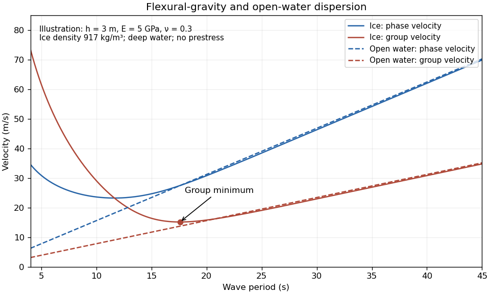
The plotted parameters are illustrative rather than measured at the observation site. They give a group-velocity minimum of a flexural-gravity wave near $15.1\mathrm{m}{\mathrm{s}}^{-1}$ at period $17.6\mathrm{s}$. There is no arbitrarily slow wave-energy branch under a continuous elastic sheet. Energy put into a localized disturbance travels away at at least this minimum group velocity; a slowly moving wind system cannot retain a wave packet indefinitely beneath itself. This reduces the opportunity for sustained local growth compared with slow, short open-water waves, and the continuous cover also prevents direct wind forcing of an exposed water surface. Incoming long swell can still propagate.

A group-velocity minimum of a flexural-gravity wave is not by itself a universal minimum wind speed for wave generation. A steadily translating forcing pattern requires a phase velocity matching its translation speed, so the minimum of $c_p$, not $c_g$, supplies the corresponding resonance threshold. Random wind forcing, dissipation and aerodynamic coupling must be specified before making an absolute generation claim.

Take $x$ positive in the off-ice wind direction, from the compact pack towards the open sea. The wind initially separates the outer ice floes, creating irregular polynyas. A larger opening gives more open-water fetch, so stronger short wind waves develop before reaching its downwind edge. Their reflection supplies a positive force on the downwind ice floes; these catch their neighbours and compact into an ice-edge band. Incoming longer swell exerts force in the opposite direction. The short waves can exert substantial force despite their smaller amplitude because a small ice floe reflects them much more effectively than it reflects the long swell.

The surface-gravity-wave energy of the short waves grows with fetch in the windward polynya, then decays rapidly across the band. Swell enters from the seaward side and usually attenuates more slowly. This gives inward forcing from the two sides: short-wave forcing is largest at the windward face and swell forcing is largest at the seaward face. In the next open polynya, short wind waves regrow from the weak transmitted component. Reflected waves also enhance energy locally on the incident side, with interference that is omitted from a smooth, phase-averaged sketch.

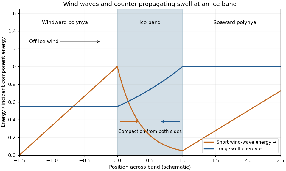
Each plotted component is normalized by its own incident energy; the curves do not assert equal absolute wind-wave and swell energies. The band is partially transmitting. For a perfectly opaque reflector, the transmitted component would instead vanish.

The initial bands have unequal floe inventories, widths and forcing. Differential drift and collisions merge some into composite bands. Larger bands tend to shield smaller downstream accumulations from the short-wave forcing needed to keep them separate, while sufficiently wide intervening polynyas can generate fresh wind waves and maintain separation. Finite available ice, available wave fetch, the opposing swell, wind strength and duration, floe size and thickness, and subsequent mergers limit the number of persistent bands. The wave-force formula alone does not select a universal count. This mechanism and its merger interpretation are supported by the original ice-band study.

There is a normalization issue in the requested stress calculation. Let $\mathcal{E}={\rho }_{w}g{a}^2/2$ be standard linear surface-gravity-wave energy for crest amplitude $a$. The deep-water wave radiation stress is $S_{xx}=\mathcal{E}/2$. Hence standard momentum balance givesFor lossless reflection with amplitude reflection coefficient $R$, $r^2=R^2{a}^2$ and $t^2=(1-R^2)a^2$, so $F_{\mathrm{phys}}={\rho }_{w}g{R}^2{a}^2/2$.

In the usual independent-floe, weak-reflection approximation, there are about $p/d$ effective layers per unit distance. Each removes a fraction $R^2$ of the forward energy, givingThis yields the intended wave-driven ice-band compaction:The attenuation approximation retains the leading term in $R^2$; an independent discrete-layer model instead gives an energy coefficient $-(p/d)\log (1-R^2)$. Neither coefficient follows from the single-object force formula without this additional scattering closure.

For ordinary crest amplitudes, the force printed in the paper is $4F_{\mathrm{phys}}$. With that printed normalization and the same attenuation law, its derivative is four times the requested stress. More generally, if $a^2=a_0^2{e}^{-\kappa x}$, the printed lossless force gives $-F^{\prime }=2{\rho }_{w}g{R}^2\kappa a^2$. Recovering the stated stress from it requires $\kappa =p{R}^2/(4d)$ instead, a different unspecified attenuation convention. The supplied force and stress cannot both be derived from standard amplitudes and the usual floe-layer attenuation law. Restoring the factor $1/4$ in the force gives a consistent intended model.

Using the printed force for the numerical question, perfect reflection gives $r=a$, $t=0$, and thereforeUsing the requested stress formula for partial reflection givesFor comparison, the consistently normalized perfect-reflection force is $50.3\mathrm{N}{\mathrm{m}}^{-1}$, and the printed force with standard attenuation would give $0.628\mathrm{N}{\mathrm{m}}^{-2}$ for the partial-reflection derivative. The approximate stress is a force per horizontal area, not a direct measure of the three-dimensional ice-skeleton stress.

The inward force gradient helps maintain a coherent, close-packed band, especially near the incident-wave faces. It is modest enough that wind, current, swell changes or mergers can disrupt the arrangement; it does not guarantee permanent mechanical stability. Perfect reflection estimates a bounding force, whereas the much smaller partial-reflection stress varies as $R^4$. No mechanical-strength law is supplied, so stability can be assessed only qualitatively.

The density-phase action of a Bose gas follows directly from $\psi =\sqrt{\rho }{e}^{i\varphi }$:The total derivative integrates to zero for periodic density. HenceA uniform density fluctuation has nonzero quadratic cost $g(\delta \rho {)}^2/2$, whereas a uniform phase change has no energy cost. Thus the radial fluctuation is massive in the static quadratic-action sense, while the phase is massless. The number-phase conjugacy term $i\delta \rho {\partial }_{\tau }\varphi$ couples their dynamics: this does not imply an additional independent gapped quasiparticle branch in the nonrelativistic Bose gas.

The compact phase winding term $i{\rho }_0\int {\partial }_{\tau }\varphi$ vanishes for the smooth zero-winding phonon sector. Globally the phase can wind by $2\pi$ while the complex field remains periodic, so that term should not be discarded across all topological sectors without a further argument.

Let $D=f_{+}^{\prime }(a)$ and write $g(t)=(f(t)-f(a))/(t-a)$ for $t>a$. By the assumed right derivative, choose $\delta >0$ with $|g(t)-D|<ϵ/2$ whenever $a<t<a+\delta$. Choose $b_0\in (a,\min (b,a+\delta ))$.

Apply the mean value theorem to $f$ on $[a,b_0]$. It gives $x\in (a,b_0)$ with $f^{\prime }(x)=g(b_0)$. Both $g(x)$ and $g(b_0)$ are within $ϵ/2$ of $D$, soThis proves the endpoint secant-tangent approximation without any continuity assumption on $f^{\prime }$. The continuity required by the theorem is only that of $f$ itself.

For continuity at any $x$, choose $\delta ={\eta }^{1/\alpha }$ for a desired error $\eta >0$. If $|y-x|<\delta$, the stated bound gives $|f(y)-f(x)|<\eta$. Thus $f$ is continuous, in fact uniformly continuous.

When $\alpha >1$, the difference quotient satisfiesTherefore the derivative exists at every point and is zero. Part (i) proves $f$ is constant. This is the lemma that Hölder exponent greater than one forces constancy; no differentiability was assumed in advance.

The mean value theorem states that a function continuous on $[p,q]$ and differentiable on $(p,q)$ has some $c\in (p,q)$ with $f(q)-f(p)=f^{\prime }(c)(q-p)$.

Take any $p<q$ inside the given open interval. Differentiability implies the continuity needed on $[p,q]$, and the derivative is zero throughout it. The mean value theorem therefore gives $f(q)=f(p)$. Since the two points were arbitrary, the function is constant on the interval.

From $f^{\prime \prime }=f$, differentiating successively gives $f^{(2r)}=f$ and $f^{(2r+1)}=f^{\prime }$ whenever those derivatives have been constructed. Starting with twice differentiability, this relation supplies the next two derivatives at each stage. Thus $f$ is infinitely differentiable, and its origin series isFor a fixed $x$, both $f$ and $f^{\prime }$ are bounded on the compact interval between zero and $x$, say by $M_x$. Every higher derivative is one of these two functions. Taylor's theorem, with the remainder just proved, therefore bounds the order-$n$ remainder by $M_x|x{|}^n/n!$, which tends to zero: its consecutive positive-term ratio is $|x|/(n+1)$. Hence the series converges to $f(x)$ for every real $x$. It also gives $f(x)=A\cosh x+B\sinh x$ by the usual hyperbolic-function series.

At any other centre $a$, apply the proved origin result to $g(t)=f(a+t)$, which also satisfies $g^{\prime \prime }=g$. Its even derivatives at zero are $f(a)$, and its odd ones are $f^{\prime }(a)$. ConsequentlyThis proves convergence at every centre without assuming that smoothness alone implies equality to a Taylor series.

For $x\ne 0$, put $P(t)={\sum }_{k=0}^{n-1}{f}^{(k)}(0)t^k/k!$ and $K=(f(x)-P(x))/x^n$. The auxiliary function $F(t)=f(t)-P(t)-K{t}^n$ satisfiesRolle's theorem first gives a zero of $F^{\prime }$ strictly between zero and $x$. Apply Rolle's theorem to $F^{\prime }$ between that zero and zero, where $F^{\prime }(0)=0$, to obtain a zero of $F^{\prime \prime }$. Continue in this way. The derivatives through order $n-1$ are continuous, since they are differentiable; hence every application is valid even if $f^{(n)}$ is not continuous. After $n$ applications there is $c$ strictly between zero and $x$ with $F^{(n)}(c)=0$.

But $F^{(n)}(c)=f^{(n)}(c)-n!K$, so $K=f^{(n)}(c)/n!$. Writing $c=\theta x$ yields the Taylor formula with Lagrange remainderThe same construction using repeated applications of Rolle's theorem applies when $x<0$, with intervals ordered from $x$ to zero. For $x=0$ the identity is immediate and any $\theta \in (0,1)$ works. This proves the Taylor theorem with Lagrange remainder using only the allowed theorem and elementary differentiation.

Use $\sin 0=0$, the derivative identity ${\sin }^{\prime }=\cos$, continuity of cosine at zero, and $\cos 0=1$. For $u\ne 0$, the mean value theorem gives $\sin u/u=\cos c_u$ for a point between zero and $u$. Hence $\sin u/u\to 1$ as $u\to 0$. For $x\ne 0$, apply this with $u=x/3^k$ to obtain the limit $\boxed{3^k\sin (x/3^k)\to x}$. For $x=0$ every term is zero.

The additional bound $|\cos t|\le 1$ and the same mean value theorem give $|\sin u|\le |u|$. ThereforeThe right side is summable. By the comparison test for series the stated series has absolute convergence for every real $x$.

The exterior derivative is an $\mathbb{R}$-linear map $d:{\Omega }^p(M)\to {\Omega }^{p+1}(M)$, agrees with the differential $df$ of a smooth function, satisfies the graded Leibniz rule $d(\alpha \wedge \beta )=d\alpha \wedge \beta +(-1{)}^p\alpha \wedge d\beta$ for $\alpha \in {\Omega }^p(M)$, and has $d^2=0$. These properties determine it locally and hence globally. To see locality directly, if a differential form $\alpha$ vanishes near $x$, choose a smooth bump function $\chi$ equal to one near $x$ and supported where $\alpha =0$. The identity $d(\chi \alpha )=d\chi \wedge \alpha +\chi d\alpha$ gives $(d\alpha {)}_x=0$. Thus global forms can be computed using local extensions in a manifold chart.

In coordinates write $\alpha ={\sum }_I{a}_{I}d{x}^{i_1}\wedge \cdots \wedge d{x}^{i_p}$. Since $d(d{x}^i)=d^2{x}^i=0$, the graded Leibniz rule forcesThis is the uniqueness of the exterior derivative from its axioms. The coordinate formula also establishes existence: it has the stated properties, and the chain rule shows that coordinate changes give the same operator.

The de Rham cohomology is the real quotient vector spaceThus a cohomology class records a closed differential form modulo an exact differential form. In degree zero there are no exact forms; closed functions are locally constant. The Poincaré lemma says that every closed form of positive degree on a star-shaped open subset of ${\mathbb{R}}^n$ is exact, and hence that positive-degree closed forms are locally exact on a smooth manifold.

For the first de Rham cohomology of the two-sphere, let $U=S^2\setminus \{N\}$ and $V=S^2\setminus \{S\}$. Stereographic projection identifies each with ${\mathbb{R}}^2$, so a closed one-form $\alpha$ has primitives $f_U,f_V$. On the connected overlap $U\cap V$, the derivative of $f_U-f_V$ is zero, so this difference is a constant. Subtracting that constant from $f_U$ makes the primitives agree. They glue to a global smooth primitive. Therefore $H_{\mathrm{dR}}^1(S^2)=0$.

Let $q:S^2\to {\mathbb{RP}}^2$ be the double covering map and $a$ the antipodal map. The pullback of a differential form identifies forms downstairs with $a$-invariant forms upstairs. Averaging $(\eta +a^{\ast }\eta )/2$ commutes with $d$. If an invariant form is exact upstairs, averaging its primitive proves it exact downstairs. Conversely an invariant cohomology class has an invariant representative by the same averaging. This proves the de Rham cohomology of a finite quotient identification $H_{\mathrm{dR}}^p({\mathbb{RP}}^2)\cong H_{\mathrm{dR}}^p(S^2{)}^{a^{\ast }}$. In degree zero the sphere is connected and $a^{\ast }$ fixes constants; degree one is zero; in degree two the granted action is multiplication by $-1$, whose invariant real subspace is zero. Forms of degree greater than two vanish. HenceThis is real de Rham cohomology; it does not detect the integral two-torsion of the real projective plane.

Here is an elementary polynomial pencil with four square members argument. Suppose first that $u,v$ are linearly dependent. Their coprimality of polynomials then forces both to be constant. Otherwise write the four distinct members as $L_j={\alpha }_{j}u+{\beta }_{j}v=s_j^2$. They are nonzero and pairwise coprime polynomials: a common nonconstant factor of two members would divide both $u$ and $v$.

Put $d=\max (\mathrm{deg}u,\mathrm{deg}v)>0$. At most one member of the pencil has degree of a polynomial smaller than $d$, since cancellation of its leading coefficient determines a unique projective pair. Choose a member $L_k$ of minimal degree $e$ and any independent member $L_l$ of degree $d$. The polynomialis nonzero: otherwise the rational function $L_k/L_l$ would have zero derivative, hence would be constant in characteristic zero. Its degree is at most $d+e-1$; if both members have degree zero the original $d>0$ assumption has already failed.

Replacing this pair by any other independent pair changes $W$ only by a nonzero scalar. Since $L_j=s_j^2$, each $s_j$ divides $W$. The pairwise coprimality of polynomials therefore gives ${\prod }_j{s}_j\mid W$. But three members have degree $d$, soa contradiction. Consequently $u$ and $v$ are constant. The possibility that a member is zero was already covered by linear dependence.

To apply this to an elliptic curve, complete the square in its Weierstrass equation of an elliptic curve and work over $\mathbb{C}$. Nonsingularity gives three distinct roots $e_1,e_2,e_3$, so the equation becomes $y^2={\prod }_{j=1}^3(x-e_j)$. A nonconstant rational parametrization of an algebraic curve would have $x=u/v$ with coprime polynomials. Clearing denominators givesThe four factors are pairwise coprime polynomials. A rational function whose square is a polynomial is itself a polynomial, by comparing numerator and denominator in lowest terms. Unique factorization, and the fact that every nonzero complex constant has a square root, make each of these four factors a square in $\mathbb{C}[t]$. They correspond to four distinct projective pairs. The result just proved forces $u,v$ to be constant, and the equation then forces $y$ to be constant as well. This proves the nonparametrizability of an elliptic curve.

We use the Van der Corput sum-integral lemma. Put $e(u)=e^{2\pi iu}$ and $I_h={\int }_a^{b}e(f(x)-hx)dx$. The Fourier series of the periodization of $1_{[a,b]}(x)e(f(x))$ giveswhere integer endpoints have half weight. This is the Dirichlet-Jordan convergence theorem for a piecewise smooth, or more generally bounded-variation, periodic function. Here $f$ is $C^1$, so the periodized function has bounded variation. Changing to the requested endpoint convention costs at most one.

Write $u=f^{\prime }$. For $h\ne 0$, $|u-h|\ge |h|-\delta >0$. Since $u$ is continuous and monotone, the reciprocal has bounded variation, and integration by parts in the Riemann-Stieltjes sense yieldsThe variation of the reciprocal is at most $2\delta /(h^2-{\delta }^2)$. Summing over $h\ne 0$ gives $O((1-\delta {)}^{-1})$, separating $|h|=1$ and using convergence of ${\sum }_{h\ge 2}{h}^{-2}$. For each endpoint, useThe symmetric partial sums of the first term are a constant multiple of ${\sum }_{h=1}^H\sin (2\pi hx)/h$, uniformly bounded in $H$ and $x$; this standard Fourier series bound follows by splitting at $h\asymp 1/\Vert x\Vert$ and applying Abel summation to the remaining sine sum. The second term is absolutely summable with bound $O((1-\delta {)}^{-1})$. The same bound therefore holds for the whole sum of the $h\ne 0$ integrals. Since $I_0$ is the ordinary integral,No second derivative is required; monotonicity supplies the needed variation estimate.

For the Hardy-Littlewood approximation to the Riemann zeta function, take $f(w)=-t\log w/(2\pi )$. On $w\ge x\ge |t|/\pi$, $|f^{\prime }(w)|\le 1/2$ and $f^{\prime }$ is monotone. The proved lemma says that the difference between the partial sum of $w^{-it}$ and its integral over $(x,Y]$ is $O(1)$ uniformly in $Y$. Weighted Abel summation with the decreasing weight $w^{-\sigma }$ then makes the weighted difference $O(x^{-\sigma })$, since its total variation on $[x,\infty )$ is $x^{-\sigma }$. Initially for $\sigma >1$, the tail integral is $x^{1-s}/(s-1)$. The bounded primitive of the discrepancy gives a locally uniformly convergent weighted discrepancy integral for every $\sigma >0$, continuing the identity to that region. Thus, away from the pole,If $t=0$ the ordinary sum-integral comparison supplies the same estimate. At $s=1$ the formula is understood meromorphically. It approximates the Riemann zeta function by a finite Dirichlet polynomial, transfers exponential sum estimates to bounds in the critical strip, yields elementary near-one bounds for $\zeta$ and its derivative, and supports estimates for the mean value of Dirichlet polynomials and numerical calculations.

Absolute convergence and the fundamental theorem of arithmetic give the Euler productFor a finite set of primes, expand the geometric factors: their product sums $n^{-s}$ over integers whose prime factors lie in that set. Let the finite sets increase through all primes. Absolute convergence permits passage to the limit and recovers the full Dirichlet series. Moreover ${\sum }_{p,m\ge 1}|p^{-ms}|/m<\infty$, so the logarithm converges and the product has no zeros there.

The same absolutely convergent logarithm, and $3+4\cos \theta +\cos 2\theta =2(1+\cos \theta {)}^2\ge 0$, giveThis is the product version of the three-four-one zero-free-region argument. It also proves there are no zeros on $\Re s=1$: if $\zeta (1+i{t}_0)=0$ for $t_0\ne 0$, its factor has order at least four as $\sigma \downarrow 1$, while the real pole contributes only order minus three and the $2t_0$ factor remains bounded. The displayed left side would tend to zero, a contradiction. At $t_0=0$ there is a pole, not a zero.

For large $|t|$, put $L=\log (|t|+2)$. The Hardy-Littlewood approximation to the Riemann zeta function at $x\asymp |t|$ gives $|\zeta (\sigma +it)|\ll L$ for $1-2/L\le \sigma \le 3$; its finite sum is bounded by ${\sum }_{n\le x}{n}^{-1+2/L}\ll L$ and the integral term is bounded. The Cauchy estimate for derivatives on circles of radius comparable to $1/L$ consequently gives $|{\zeta }^{\prime }(\sigma +it)|\ll L^2$ for $1-L^{-9}\le \sigma \le 2$.

Take ${\sigma }_0=1+a{L}^{-9}$ with a small fixed $a>0$. The product inequality, $\zeta ({\sigma }_0)\ll L^9/a$, and $|\zeta ({\sigma }_0+2it)|\ll L$ implyIf $1-c{L}^{-9}\le \sigma \le {\sigma }_0$, integration of the derivative along the horizontal segment changes this value by at most $C(a+c)L^{-7}$. Choose $a$ sufficiently small that $Ca<c_0{a}^{3/4}/4$, then $c\le a$ sufficiently small. The lower bound remains a positive multiple of $L^{-7}$. For ${\sigma }_0\le \sigma \le 2$, the same product inequality, $\zeta (\sigma )\le \zeta ({\sigma }_0)$, and the near-one upper bound give that lower bound directly. For $\sigma \ge 2$, the reciprocal Euler product gives $|1/\zeta (s)|\le \zeta (2)$.

Finally the no-zero result on $\Re s=1$, compactness at bounded heights and the regular reciprocal at the pole allow a further fixed reduction of $c$ to include bounded $t$. We have proved the weak logarithmic zero-free region for the Riemann zeta functionThe reciprocal at $s=1$ is its holomorphic extension, equal to zero.