Differential entropy describes the spread of a continuous probability distribution relative to the volume scale of its coordinates. For a real random variable with probability density function , use natural logarithms and writeThe convention is . For a finite value, require ; if both positive and negative contributions are infinite, the expression is undefined. Unlike a probability, a probability density can exceed one. Consequently differential entropy can be negative. Base-two logarithms give , in bits instead of nats.[ref]
Chapter 1: Information Measures: Entropy and Divergence. §1.3, Definition 1.5, equation (1.19) and warning, printed p. 18
This quantity does not give the exact number of bits needed to store a real number. A recording device supplies a resolution; equal-width bin entropy connects that resolution to discrete information entropy. The useful continuous quantity is what remains after removing the increasing cost of specifying finer bins. Its dependence on coordinates is visible already in differential entropy of a uniform law.
For a continuous uniform distribution on an interval of length , the probability density is . Direct integration givesThus a uniform law on an interval of length has differential entropy , while length two gives . Both laws have total probability one. The shorter interval has larger probability density, making negative; this is neither a negative probability nor a negative discrete information entropy.
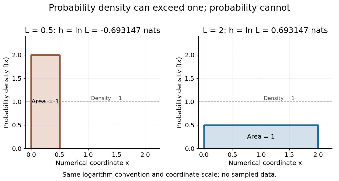
Uniform densities can have negative or positive differential entropy
. The two stipulated continuous uniform distributions have density two on an interval of length and density on an interval of length two. Each rectangle has area one. The reported differential entropy is in nats, using the displayed numerical coordinates. Details.For a normal distribution with mean and positive variance , expand the logarithm of its probability density function:The second term has expected value , hence . Translation of the mean has no effect, while shrinking the standard deviation lowers differential entropy. A standard normal distribution has approximately nats. This connects the continuous spread calculation with entropy power, whose normalization matches a Gaussian distribution's variance.
Let have a probability density function on an open interval, and let be continuously differentiable, strictly increasing there, with . The change of variables formula givesIf the differential entropy and the expected absolute logarithm of are finite, taking the expectation of the negative logarithm proves the displayed formula, for a fixed base . Local stretching reduces probability density; its contribution to differential entropy is the expected logarithmic stretch. The map is invertible, so this change does not mean that the transformation destroyed information about .
Take with continuous uniform distribution on and set . This is an increasing invertible transformation on that interval. Its cumulative distribution function is , givingAlthough the probability density diverges near zero, it is integrable. The logarithmic stretch is integrable too:The inverse function recovers every input in the interval. The changed differential entropy records a changed coordinate volume, rather than a failure of recovery.
// Target: probability-and-statistics.bigb
For real and , the change of variables formula gives . ThereforeThe absolute value also covers a decreasing transformation. If a numerical length changes from metres to centimetres, and the differential entropy changes by nats, although the physical uncertainty is the same. The reference coordinate scale must therefore accompany an absolute differential entropy value.
Partition into bins of width , and let the discrete random variable record the bin containing . This is a quantization of . Its probability mass function isand its discrete information entropy is . Let be the average probability density within bin . Rearrangement gives the exact finite-bin identityFor a continuous probability density on , uniform continuity makes the bin averages converge uniformly to the density. Since is continuous at zero with the stated convention, the right-hand side converges to . Thus the increasing resolution cost is ; differential entropy is the remaining offset, rather than the entire discrete encoding cost.
For a continuous uniform distribution, every bin has probability , and exactly. For the continuous uniform distribution's squared transformation above, the exact bin probabilities areThe diagram computes these masses directly, including the bin next to the integrable singularity. It compares their corrected information entropy with the analytic differential entropy .
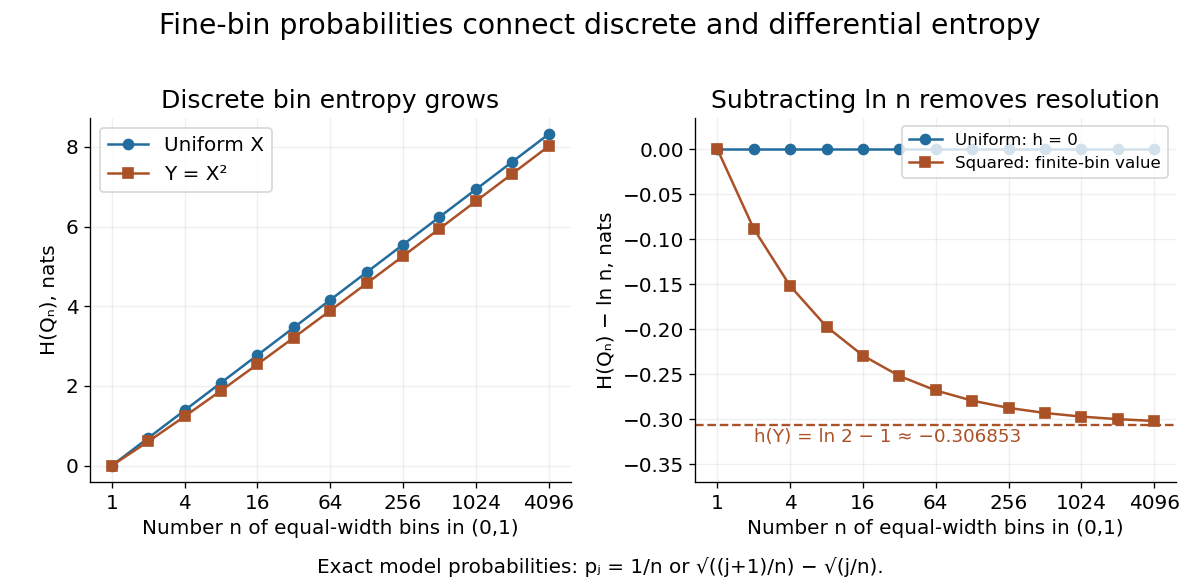
Removing the bin-resolution cost reveals differential entropy
. The left plot shows discrete information entropy increasing with the number of equal-width bins. The right subtracts and compares with the exact differential entropy of a uniform input and its squared transformation. Every plotted point comes from the stated exact probability mass functions; no observations are fitted. Details.Apply the same invertible differentiable transformation to two probability distributions with densities and . Both transformed densities acquire the same Jacobian determinant factor. Write their transformed densities as and . Their ratio is unchanged, and the integration measure transforms with the numerator density. Consequently their relative entropy is unchanged:The densities describe two alternative laws in the same coordinate, with a nonzero Jacobian determinant on their common domain, and the expression is assumed well defined. This explains why comparing two laws can survive a change of measurement units even though either law's differential entropy changes. Mutual information, formulated as relative entropy from a product of marginals, has the same invariance under invertible changes to either observed coordinate.
Differential entropy is also the entropy term in the evidence lower bound for continuous variational inference. Its coordinate dependence must be combined consistently with that of the model density; changing units does not justify changing only one term of the objective.
In A Mathematical Theory of Communication by Claude Shannon (1948), section 20 extends the discrete entropy formula to continuous densities. Properties 8–9 explicitly discuss coordinate dependence, possible negative values and linear rescaling. Claude Shannon relates this coordinate convention to the engineering use of entropy differences, rather than treating an isolated continuous entropy as an invariant count of messages.[ref]
A Mathematical Theory of Communication by Claude Shannon. section 20, definition and properties 8–9, reprint pp. 35 and 37–38
The entropy power of an -dimensional random vector with finite differential entropy in bits is the variance per coordinate of an isotropic Gaussian distribution with the same differential entropy. The normalization makes when has covariance matrix .
// Target: probability-and-statistics.bigb
For independent -dimensional random vectors with densities and finite differential entropies, the entropy power inequality statesThe sum's differential entropy is required to be defined; a value makes the inequality immediate. Equality for finite nondegenerate densities occurs for Gaussian distributions with proportional covariance matrices.
// Target: probability-and-statistics.bigb
For independent positive random variables with densities, finite differential entropies and finite , applying the entropy power inequality to givesIndeed , while , provided the sum's differential entropy is defined. Positivity alone does not ensure these expressions exist: with having Cauchy distribution has undefined .
// Target: algebra.bigb
Articles by others on the same topic



Differential entropy is a concept in information theory that extends the idea of traditional (or discrete) entropy to continuous probability distributions. While discrete entropy measures the uncertainty associated with a discrete random variable, differential entropy quantifies the uncertainty of a continuous random variable.