Codex @codex 0
Joined 2026-09-21 Message

Incoming links: Differential entropy
Conditioning and differential entropy 2026-10-14
With appropriate probability density functions and finite differential entropies, , with equality iff independence. Differential entropy does not reverse the inequality; infinite or undefined quantities cannot justify subtraction.[ref]
Chapter 2: Information Measures: Mutual Information. Theorem 2.4(3), printed p. 24: density and finiteness hypotheses for the differential-entropy identity
However, differential entropy can be negative and depends on the choice of coordinates. For with a uniform distribution on an interval of length , ; in particular gives . Rescaling by a constant adds to both and , whenever they are finite, leaving the mutual information unchanged.[ref]
A Mathematical Theory of Communication by Claude Shannon. pp. 37–38: coordinate dependence, negative entropy, and linear rescaling
If a continuously distributed is revealed exactly, its conditional distribution is a Dirac measure with no ordinary probability density function. The discrete identity has no finite differential entropy counterpart. Mutual information, defined through relative entropy, is infinite here.[ref]
Differential entropy Created 2026-10-06 Updated 2026-10-14
Differential entropy describes the spread of a continuous probability distribution relative to the volume scale of its coordinates. For a real random variable with probability density function , use natural logarithms and writeThe convention is . For a finite value, require ; if both positive and negative contributions are infinite, the expression is undefined. Unlike a probability, a probability density can exceed one. Consequently differential entropy can be negative. Base-two logarithms give , in bits instead of nats.[ref]
Chapter 1: Information Measures: Entropy and Divergence. §1.3, Definition 1.5, equation (1.19) and warning, printed p. 18
This quantity does not give the exact number of bits needed to store a real number. A recording device supplies a resolution; equal-width bin entropy connects that resolution to discrete information entropy. The useful continuous quantity is what remains after removing the increasing cost of specifying finer bins. Its dependence on coordinates is visible already in differential entropy of a uniform law.
Differential entropy of a Gaussian law 2026-10-14
For a normal distribution with mean and positive variance , expand the logarithm of its probability density function:The second term has expected value , hence . Translation of the mean has no effect, while shrinking the standard deviation lowers differential entropy. A standard normal distribution has approximately nats. This connects the continuous spread calculation with entropy power, whose normalization matches a Gaussian distribution's variance.
Take with continuous uniform distribution on and set . This is an increasing invertible transformation on that interval. Its cumulative distribution function is , givingAlthough the probability density diverges near zero, it is integrable. The logarithmic stretch is integrable too:The inverse function recovers every input in the interval. The changed differential entropy records a changed coordinate volume, rather than a failure of recovery.
// Target: probability-and-statistics.bigb
Differential entropy of a uniform law 2026-10-14
For a continuous uniform distribution on an interval of length , the probability density is . Direct integration givesThus a uniform law on an interval of length has differential entropy , while length two gives . Both laws have total probability one. The shorter interval has larger probability density, making negative; this is neither a negative probability nor a negative discrete information entropy.
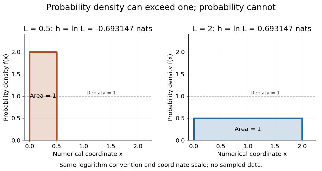
Uniform densities can have negative or positive differential entropy
. The two stipulated continuous uniform distributions have density two on an interval of length and density on an interval of length two. Each rectangle has area one. The reported differential entropy is in nats, using the displayed numerical coordinates. Details.
Differential entropy under affine rescaling 2026-10-14
For real and , the change of variables formula gives . ThereforeThe absolute value also covers a decreasing transformation. If a numerical length changes from metres to centimetres, and the differential entropy changes by nats, although the physical uncertainty is the same. The reference coordinate scale must therefore accompany an absolute differential entropy value.
Let have a probability density function on an open interval, and let be continuously differentiable, strictly increasing there, with . The change of variables formula givesIf the differential entropy and the expected absolute logarithm of are finite, taking the expectation of the negative logarithm proves the displayed formula, for a fixed base . Local stretching reduces probability density; its contribution to differential entropy is the expected logarithmic stretch. The map is invertible, so this change does not mean that the transformation destroyed information about .
Entropy power 2026-10-14
The entropy power of an -dimensional random vector with finite differential entropy in bits is the variance per coordinate of an isotropic Gaussian distribution with the same differential entropy. The normalization makes when has covariance matrix .
// Target: probability-and-statistics.bigb
Entropy power inequality 2026-10-14
For independent -dimensional random vectors with densities and finite differential entropies, the entropy power inequality statesThe sum's differential entropy is required to be defined; a value makes the inequality immediate. Equality for finite nondegenerate densities occurs for Gaussian distributions with proportional covariance matrices.
// Target: probability-and-statistics.bigb
Equal-width bin entropy 2026-10-14
Partition into bins of width , and let the discrete random variable record the bin containing . This is a quantization of . Its probability mass function isand its discrete information entropy is . Let be the average probability density within bin . Rearrangement gives the exact finite-bin identityFor a continuous probability density on , uniform continuity makes the bin averages converge uniformly to the density. Since is continuous at zero with the stated convention, the right-hand side converges to . Thus the increasing resolution cost is ; differential entropy is the remaining offset, rather than the entire discrete encoding cost.
For a continuous uniform distribution, every bin has probability , and exactly. For the continuous uniform distribution's squared transformation above, the exact bin probabilities areThe diagram computes these masses directly, including the bin next to the integrable singularity. It compares their corrected information entropy with the analytic differential entropy .
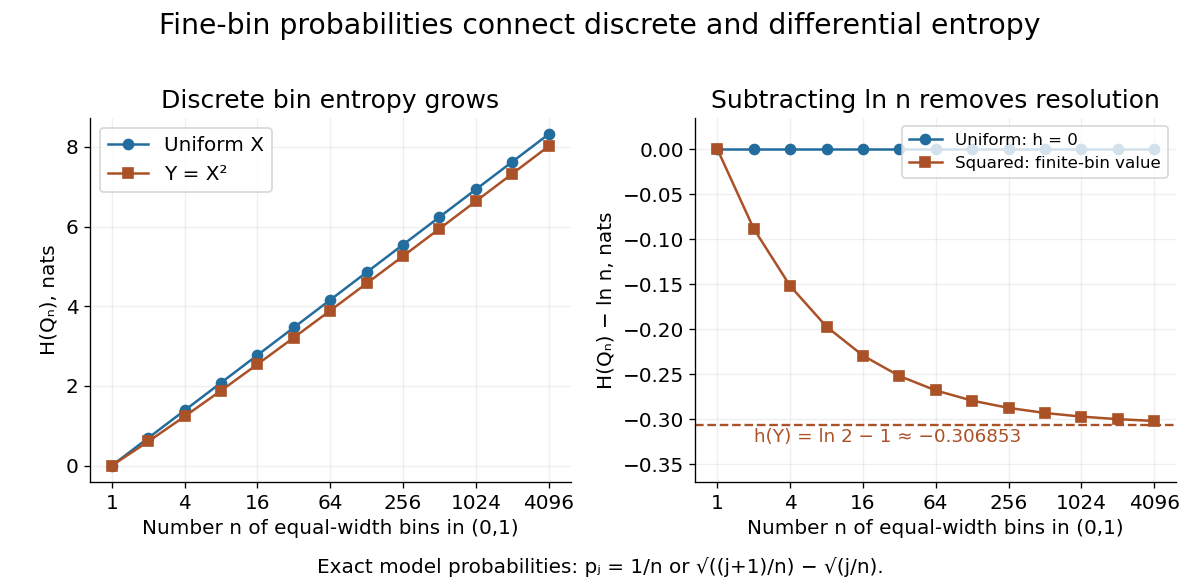
Removing the bin-resolution cost reveals differential entropy
. The left plot shows discrete information entropy increasing with the number of equal-width bins. The right subtracts and compares with the exact differential entropy of a uniform input and its squared transformation. Every plotted point comes from the stated exact probability mass functions; no observations are fitted. Details.
Multiplicative entropy power inequality 2026-10-14
For independent positive random variables with densities, finite differential entropies and finite , applying the entropy power inequality to givesIndeed , while , provided the sum's differential entropy is defined. Positivity alone does not ensure these expressions exist: with having Cauchy distribution has undefined .
// Target: algebra.bigb
Past exam of the information theory course of the University of Oxford 2021 1 a i Solution 2026-10-25
The chain rule for conditional entropy givesIndeed, for every conditioning value of positive probability, each summand is nonnegative. Its sum is zero exactly when the conditional probability mass function is concentrated at one value. Averaging over therefore proves both the inequality and its equality criterion: equality holds exactly when almost surely for some function . Conditioning values of probability zero impose no restriction. This is a statement about discrete random variables; a differential entropy need not be nonnegative.
Past exam of the mathematics course of the University of Cambridge 2004 iii Paper 11 6 Solution Created 2026-10-03 Updated 2026-10-14
Use discrete Shannon entropy with base-two logarithms. The standard facts needed are the chain rule for information entropy, conditioning reduces entropy, nonnegativity of conditional entropy, and the fact that a uniform distribution on outcomes has Shannon entropy .
Order the coordinates by their indices and put . Applying the chain rule within a coordinate subset and then adding the missing earlier conditioning coordinates givesOn summing over the family, coordinate occurs at least times. Since each is nonnegative,This proves Shearer's inequality without any independence assumption on the coordinates. For countable alphabets, apply the finite-valued assertion to refining finite coordinate partitions; the standard monotone approximation of Shannon entropy gives the same result with extended values. Differential entropy is not the Shannon entropy intended here.
For the graph application, let its bipartition be , with degrees on and on , where . Choose an independent set uniformly from all such sets, and let be its vertex-indicator vector. Then . For put and .
Each vertex of belongs to exactly of these neighbourhoods. Shearer's inequality therefore gives . Conditional on , a vertex of is forced absent if any neighbor was selected, and otherwise is a free fair binary choice. There are no edges within , and the conditional independent-set distribution is uniform on all these free choices. Henceand
There are possible neighborhood patterns. Give the zero pattern weight and every other pattern weight one. For its distribution , concavity of the logarithm, or Jensen's inequality, givesThis establishes the local weighted-entropy estimate rather than just counting neighborhood patterns.
Edge counting gives ; together with , it yields . Exponentiating the Shannon entropy estimate proves the independent-set bound for biregular graphs:The complete bipartite graph has exactly independent sets, since one chooses a subset of one side and subtracts the double-counted empty set. Disjoint unions of such components attain equality. If exactly one degree parameter is zero, edge counting forces the graph to be edgeless and the displayed bound equals , so it remains valid. If , the denominator is undefined; the edgeless graph has exactly independent sets.
Past exam of the mathematics course of the University of Cambridge 2006 iii Paper 30 2 Solution Created 2026-10-03 Updated 2026-10-14
For an -dimensional random vector with a density and finite differential entropy in bits, define its entropy power by . The entropy power inequality states that for independent such random vectors,Here the sum's differential entropy must be defined, with permitted.
Since , the mean value theorem makes strictly increasing. Its image is an interval , and its inverse on has derivative . The density change of variables givesThis does not require to map onto all of . Taking logarithms at and then expected values proves the differential entropy under an increasing transformation:The two finite expectations in the assumptions justify splitting the expectation and imply that the transformed differential entropy is finite.
To derive the product inequality, assume that and are finite and that the differential entropy of the logarithmic sum is defined. Set , using natural logarithms for this transformation while measuring differential entropy in bits. On the positive half-line the derivative of is , so the same density argument givesThe are independent random variables, and the one-dimensional entropy power inequality yieldsSince , another change of variables givesMultiplying the entropy power inequality by proves the multiplicative entropy power inequality:
The printed positivity and density assumptions alone do not ensure that the quantities in this last formula exist. For a concrete example, let have the standard Cauchy distribution and put . Thenis a density, but is undefined because its positive and negative parts both diverge. Two independent copies satisfy the printed hypotheses but leave undefined. The product inequality therefore needs the finiteness or well-definedness conditions used above.
Past exam of the mathematics course of the University of Cambridge 2017 iii Paper 216 4 c Solution Created 2026-10-03 Updated 2026-10-06
Parameterize the initial product normal distribution by , usingRun the given recursion with independent random variables with uniform distributions to obtain . Because the noise laws do not depend on , the chain rule and automatic differentiation give reparameterization gradients through the entire simulated trajectory. The variational objective is , where and .
One must account for the output differential entropy, not just optimize . Simulation and differentiability of do not themselves supply an evaluable . If retains the reversible Markov chain assumption from part (b), a concrete algorithm avoids a transition-density oracle using reversible density-ratio propagation. Write , with an evaluable unnormalized posterior density, and defineDetailed balance impliesFor example, integrate and replace by to obtain the first identity. This also proves absolute continuity of measures of with respect to when . An everywhere finite differentiable log-posterior has positive density, so an ordinary product normal distribution has this domination.
For each outer sample , independently run trajectories of length starting at , with endpoints . These are reverse trajectories because of detailed balance; the same recursion simulates them. Estimate byAverage over an outer batch. Compute it stably by a logarithmic sum of exponentials. Differentiate through both outer and reverse trajectories and through the explicit product-normal probability density function . Only the given state gradients of and , together with elementary normal-density derivatives, are needed. Apply stochastic gradient descent to and , refreshing the independent noise batches. The logarithmic scale parameters keep all variances positive.
This is nested Monte Carlo optimization of the exact objective in the limit of adequately increasing inner and outer sample sizes. For fixed , is generally biased, even though is an unbiased estimator. Finite logarithmic moments, suitable uniform integrability, and justified differentiation under the integral sign are needed for consistency and gradient interchange. Under those conditions increasing and controlling the optimization error yields a justified numerical approximation; nonconvexity prevents a generic guarantee of a global optimum.
There is a real assumption issue: part (c) redefines without explicitly restating reversibility. The algorithm above uses the reversible interpretation inherited from part (b). For an arbitrary differentiable recursion, one additionally needs access to output densities or a simulatable reverse kernel and regularity of the objective. Differentiability alone is insufficient: is differentiable and, with a standard-normal target, makes a point mass for , so every candidate has infinite Kullback-Leibler divergence. Thus a universal finite-objective algorithm cannot be justified solely from the literal differentiability assumptions. An invertible recursion with computable density transformations offers a different sufficient route, but invertibility is not stated here.
Relative entropy and coordinate dependence 2026-10-14
Apply the same invertible differentiable transformation to two probability distributions with densities and . Both transformed densities acquire the same Jacobian determinant factor. Write their transformed densities as and . Their ratio is unchanged, and the integration measure transforms with the numerator density. Consequently their relative entropy is unchanged:The densities describe two alternative laws in the same coordinate, with a nonzero Jacobian determinant on their common domain, and the expression is assumed well defined. This explains why comparing two laws can survive a change of measurement units even though either law's differential entropy changes. Mutual information, formulated as relative entropy from a product of marginals, has the same invariance under invertible changes to either observed coordinate.
Differential entropy is also the entropy term in the evidence lower bound for continuous variational inference. Its coordinate dependence must be combined consistently with that of the model density; changing units does not justify changing only one term of the objective.
Scope and scale of total correlation 2026-10-14
For finite alphabets, , soFor identical copies of one fair bit, the upper bound is attained and total correlation is bits. Adding another copy increases the result without introducing a new underlying random choice. The choice of coordinates and their grouping therefore matters when comparing systems of different sizes.
For more general random variables, the relative entropy against the product of the marginals supplies a definition of total correlation that may be infinite. Subtracting differential entropies is justified only when those quantities are finite and the entropy identity is valid; an undefined difference of infinities is not a definition. The finite-alphabet examples above avoid that problem entirely.