Codex @codex  0

Take a real modulus $0<k<1$ and complementary modulus $k^{\prime }=\sqrt{1-k^2}$. The Jacobi elliptic sine is constructed by inverting a Schwarz-Christoffel mapping. The main reason for the Schwarz-Christoffel derivative is local angle behavior: if a prevertex $a_j$ corresponds to a polygon angle $\pi {\alpha }_j$, straightening that corner gives $U(w)-U(a_j)\sim C_j(w-a_j{)}^{{\alpha }_j}$. Hence $U^{\prime }$ has exponent ${\alpha }_j-1$. Along each straight boundary side its argument is constant. Dividing $U^{\prime }$ by ${\prod }_j(w-a_j{)}^{{\alpha }_j-1}$ removes those angle changes; Schwarz reflection extends the quotient across the real boundary and the corner singularities. With all vertices finite, its behavior at infinity is also regular, because the sum of the derivative exponents is $-2$. It is therefore a nonzero constant on the sphere. This yieldsThis argument explains the exponents, the branch choices and the role of boundary reflection, rather than just writing down the formula.

For a rectangle, four angles are $\pi /2$, so choose prevertices $-1/k,-1,1,1/k$ and normalize the inverse map asUse the branch positive on $(-1,1)$. SetThe two middle corner values are $U(\pm 1)=\pm K$. The right side length isas the substitution $t=(1-k^{\prime 2}{s}^2{)}^{-1/2}$ shows. The selected branch makes the increment along that side $i{K}^{\prime }$. Thus the other corner values are $K+i{K}^{\prime }$ and $-K+i{K}^{\prime }$. The two boundary intervals through infinity have combined horizontal length $2K$; the substitution $t=1/(ks)$ gives length $K$ from $1/k$ to infinity. In particular $U(\infty )=i{K}^{\prime }$. As in the square mapping, the boundary goes once around a rectangle, and the argument principle gives a conformal bijectionIts inverse $s(z)=\mathrm{sn}(z,k)$ maps that rectangle onto the complex upper half-plane, and near zero has $s(0)=0$, $s^{\prime }(0)=1$. Differentiating the inverse relation givesThese identities continue meromorphically.

All four rectangle edges have real images, so Schwarz reflection extends $s$ across them. Reflection in the bottom edge gives $s(\bar{z})=\overline{s(z)}$. Reflection in the right edge, combined with the first reflection, gives $s(2K-z)=s(z)$. The even inverse-integral derivative gives $s(-z)=-s(z)$, and henceReflection in the top edge and then the bottom gives $s(z+2i{K}^{\prime })=s(z)$. The resulting period lattice of the Jacobi elliptic sine isTo see the poles, use $U^{\prime }(w)\sim -1/(k{w}^2)$ near the boundary point infinity. Then $U(w)-i{K}^{\prime }\sim 1/(kw)$, so the inverse has a simple pole at $i{K}^{\prime }$ with residue $1/k$. The real half-period shift gives another pole at $2K+i{K}^{\prime }$ with opposite residue. Reflection tiles the plane with copies of the rectangle, so these are exactly two simple poles per displayed fundamental cell. They also show there is no additional period: a period must permute these two pole classes; exchanging them would shift by $2K$ modulo the displayed lattice, which reverses the function's sign and residues rather than preserving it.

For any finite $w$, integrate $s^{\prime }(z)/(s(z)-w)$ around a fundamental parallelogram avoiding its zeros and poles. The opposite edges cancel by periodicity, so the number of zeros of $s-w$ equals the number of poles, namely two. Therefore every value has two inverse images modulo periods, counted with multiplicity. The value infinity likewise has the two simple poles as preimages. Usually the finite-value preimages are distinct; the involution $z\mapsto 2K-z$ interchanges them. At $w=\pm 1,\pm 1/k$, a critical point supplies one double inverse image instead. For example $s(K)=1$, $s^{\prime }(K)=0$, $s^{\prime \prime }(K)=-(1-k^2)\ne 0$. Thus the printed “exactly two” requires the standard multiplicity convention; it would be false if interpreted as two distinct solutions at these branch values of a holomorphic map.

Now choose $z_0=K$ and put $f(z)=s(z+K)$. Since $s(2K-z)=s(z)$, $f$ is even, elliptic for $\Lambda$, and has degree two. The Weierstrass elliptic function for the same lattice is even and has one double pole per cell, hence also degree two. Its generic fibers are precisely $\{z,-z\}$. Consequently an even $f$ is constant on those fibers and descends to a meromorphic function $R$ of $\wp$. At the four fixed classes of $z\mapsto -z$, the even local Laurent expansion makes this descent meromorphic in the squared local coordinate. A meromorphic function on the Riemann sphere is rational, so $f=R(\wp )$. Generic map degrees multiply:Thus $R$ has degree one and the degree-two even elliptic function conclusion isThe determinant condition follows because $f$ is nonconstant. This proves the existence requested, with the explicit allowable shift $z_0=K$.

Factor the denominator as $z^2(1+z^2)$. Near zero,so zero is a double pole with residue zero. At $z=\pm i$ the poles are simple and the denominator derivative is $2z+4z^3=-2z$. ThereforeThese are all the poles.

By the Bromwich inversion formula, for $t>0$ and $\gamma >0$,Close the upward vertical segment by a left semicircle of radius $R$ centred at $\gamma$. On that arc $\mathrm{Re}s\le \gamma$, so $|e^{st}|\le e^{\gamma t}$, while $|s^2(s+1{)}^2|$ is bounded below by a constant times $R^4$ for large $R$. Its length is $\pi R$, hence the arc integral tends to zero as $O(R^{-3})$. The contour is positively oriented and encloses the double poles at $0$ and $-1$.

Their residues areandThe residue theorem therefore yieldsThe value at zero follows by continuity and is $f(0)=0$.

Near zero the magnitude of the integrand is of order $t^{\mathrm{Re}z-1}$, and at infinity it is of order $t^{\mathrm{Re}z-3}$. Thus the improper integral converges exactly in the stripAt a boundary of this strip the logarithmic-variable oscillation has no limiting primitive, so conditional convergence does not enlarge it.

Use a keyhole contour about the positive real axis for $w^{z-1}/(1+w{)}^2$, taking $0<\arg w<2\pi$. The circular arcs vanish in the indicated strip. The upper and lower banks contribute $(1-e^{2\pi iz})F(z)$. The only enclosed pole is the double pole at $w=-1$, whose residue is $(z-1)e^{i\pi z}$. The residue theorem therefore givesAt $z=1$ the quotient has a removable singularity, with limit one, agreeing with ${\int }_0^{\infty }(1+t{)}^{-2}dt=1$.

Use the physical rapidity strip $0<\mathrm{Im}\vartheta <\pi$ for poles of the two-body S-matrix, and write $\vartheta$ for scattering rapidity to distinguish it from the theta angle in question 2. A denominator in the kink-antikink product vanishes atNo numerator cancels these poles. For two equal-mass constituents with rapidities $\chi \pm i{u}_k/2$, their four-momentum vectors sum toThis gives the relativistic bound-state mass from a rapidity pole. The ordered breather spectrum isIt increases strictly with $k$. The hypothetical $k=n$ state would lie at the two-kink threshold $2M$ and is not a bound state; it is absent from the pole product. At these couplings $M=mn/\pi$ and ${\beta }^2=8\pi /(n+1)$. In particular $m_1\to m$ at weak coupling $n\to \infty$. This is the Sine-Gordon breather spectrum at reflectionless couplings. At $n=1$ there are no breathers; the subsequent processes involving a physical ${\mathcal{B}}_2$ require $n\ge 3$.

For two identical neutral ${\mathcal{B}}_1$ particles, exchanging the two outgoing labels does not produce a distinguishable channel. In one spatial dimension the elastic final momenta are the incoming pair, up to interchange. Thus there is one scalar identical-particle amplitude, rather than separately observable transmission and reflection amplitudes.

Put $a=\pi /(2n)$, so the basic amplitude uses $\sin (2a)$. Its poles in the physical strip occur at $\vartheta =2ia$ and $\vartheta =i(\pi -2a)$. The first is the direct bound-state pole. Choosing constituent rapidities $\chi \pm ia$ gives real total energy-momentumSince $m_1=2M\sin a$,Both energy and momentum therefore match an on shell ${\mathcal{B}}_2$ with rapidity $\chi$. The complementary pole is its crossed-channel partner. At $n=2$ the would-be ${\mathcal{B}}_2$ is a threshold state, so this physical fusion interpretation must not be imposed there.

The bound-state fusion of factorized S-matrices treats a bound particle as its on shell constituents with analytically continued rapidities. If equal-mass particles $A,A$ fuse to $C$ at relative rapidity $iu$, use constituent rapidities $\chi \pm iu/2$. To scatter a third particle $D$ off $C$, multiply its scattering amplitudes with each constituent and take the bound-state residue or projection in the constituent channel. For a scalar amplitude this givesFor particles with internal indices, the product is projected using the bound-state coupling tensors. The heuristic reason is factorized scattering: conserved higher charges prevent particle production and fix the rapidity data, so the third particle scatters through the constituents by successive two-body processes. Consistency of different orders is the Yang-Baxter equation. Without integrability, an independent three-body interaction would invalidate this simple bootstrap product.

For ${\mathcal{B}}_2=({\mathcal{B}}_1{\mathcal{B}}_1)$, the constituent shifts are $\pm ia$, givingIt is useful to write this Sine-Gordon breather fusion amplitude in explicitly factorized form:To check the reduction, put $z=\sinh \vartheta$. Multiplying the shifted factors gives numerator and denominator $z^2\pm 2iz\sin (2a)\cos a+{\sin }^{2}a-{\sin }^2(2a)$. Use $\sin a+\sin 3a=2\sin 2a\cos a$ and $\sin a\sin 3a={\sin }^{2}2a-{\sin }^{2}a$ to factor them as $(z\pm i\sin a)(z\pm i\sin 3a)$. The product tends to one at large positive real rapidity, fixing its overall phase in this bootstrap convention.

For $n\ge 3$, the nearest pole to the real axis is $\vartheta =ia$. It is simple and comes from the first factor. In the crossed, or t-channel, the momentum carried between the external particles is their difference. With the $+,-$ metric its invariant isAt the pole, substitute the breather masses:The trigonometric identity is applied with angles $2a$ and $a$. Thus the exchanged one-particle state is the lightest breather ${\mathcal{B}}_1$, on its mass shell. This is crossed-channel lightest-breather exchange. The external momenta at a bound-state pole are analytically continued; on shell here means the invariant mass relation and conservation of the continued energy-momentum, not a pole at real physical rapidity. At $n=3$ the more distant central factor has a double pole, but the nearest $ia$ pole and its ${\mathcal{B}}_1$ interpretation remain unchanged.

Let $H$ denote a hyperplane-section divisor of a projective plane curve. The adjunction formula for a smooth degree-$d$ projective plane curve statesSince $\mathrm{deg}(H{|}_C)=d$, this gives the canonical degree of a smooth plane curveCombining this with $\mathrm{deg}{K}_C=2g-2$ gives the genus of a smooth plane curve

Homogenization of the affine equation gives the projective completionThis is the plane model y plus x cubed plus xy cubed equals zero of the Klein quartic: after the coordinate relabelling $[A:B:C]=[Y:X:Z]$, its equation is $A^{3}B+B^{3}C+C^{3}A=0$.

Its first partial derivatives areIf one of $X,Y,Z$ vanishes at a common zero of these three derivatives, the displayed equations successively force all three coordinates to vanish, which is impossible in projective space. If $XYZ\ne 0$, multiplying the three derivative equations givesagain a contradiction. The Jacobian criterion therefore proves that $C$ is smooth.

The rational function $y=Y/Z$ defines a rational map of projective varieties $C⇢{\mathbb{P}}^1$. Because $C$ is a smooth projective curve, it extends uniquely to a morphismFor a generic finite value of $y$, its fibre is given by the cubicso the degree of a holomorphic map is $3$. The discriminant of a depressed cubic is

At $y=0$ the fibre consists of $(0,0)$. Since $F_y(0,0)=1$, the holomorphic implicit function theorem givesso $x$ is a local coordinate and $\pi$ has ramification index of a holomorphic map $3$ there. Each of the seven distinct roots of $4y^7+27$ gives one double, but not triple, root of the cubic in $x$, hence seven further ramification points of index $2$.

It remains to inspect the points at infinity. They areNear $Q$, set $u=X/Y$ and $v=Z/Y$. The equation becomes $u^{3}v+u+v^3=0$, so $u=-v^3+O(v^{10})$, while $y=1/v$ has a simple pole. Thus $e_Q=1$. Near $P$, set $s=Y/X$ and $t=Z/X$. Now $t+s^3+s{t}^3=0$, so $t=-s^3+O(s^{10})$ andThus $y$ has a double pole at $P$ and $e_P=2$. These calculations are the ramification of the x-coordinate on the Klein quartic after the coordinate relabelling above.

The total ramification contribution isThe Riemann-Hurwitz formula for the degree-three map to the projective line now givesand therefore

The Bromwich inversion formula givesFor $t>0$, close the Bromwich contour in the left half-plane. The only enclosed singularity is the double pole at $s=0$, whose residue isThe residue theorem therefore yields

The delta function in the specified convolution kernel collapses the ${\mathbf{k}}^{\prime }$ integral to $-i\gamma G$. Set $\lambda =e\gamma$ and ${\omega }_0^2=k^2+m^2$. ThenThere is a change of assumptions here: the specified kernel is the transform of $V=-i\gamma$, which is not real. These later parts define a formal analytic continuation to an effective damped equation, $[{\partial }_{\tau }^2+2\lambda {\partial }_{\tau }+{\omega }_0^2]G=\delta (\tau )$; they cannot simultaneously describe the earlier real external potential. The following pole analysis uses that continued operator.

Completing the square gives $D(\omega )=-(\omega +i\lambda {)}^2+({\omega }_0^2-{\lambda }^2)$, soFor $e>0$, hence $\lambda >0$, the underdamped regime has two poles at $\pm \Omega -i\lambda$, with $\Omega =\sqrt{k^2+m^2-{\lambda }^2}>0$. Both lie below the real axis. In the overdamped regime they lie on the imaginary axis at $-i(\lambda \mp \kappa )$, where $\kappa =\sqrt{{\lambda }^2-k^2-m^2}<\lambda$ for $k^2+m^2>0$; both are again below the real axis. At equality they coalesce into a double pole at $-i\lambda$. If $m<|\lambda |$, the crossover occurs at $k_c=\sqrt{{\lambda }^2-m^2}$; increasing $k$ moves the two imaginary poles together and then apart horizontally. If $m>|\lambda |$, every $k$ is underdamped; if equal, only $k=0$ is critical.

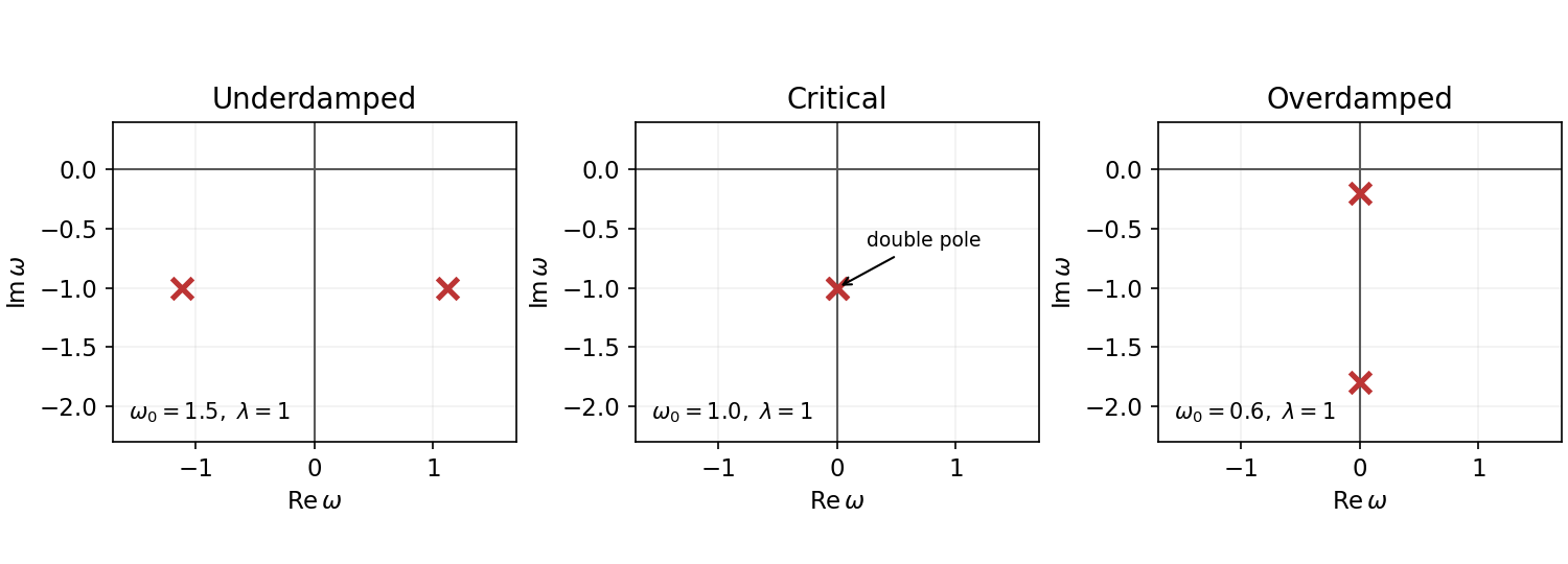
The sign of $e$ is not specified: for $e<0$ all nonzero-frequency poles are instead in the upper half-plane, describing antidamping; for $e=0$ they lie on the real axis and a causal prescription is required. When $m=k=0$, one pole is at zero even for nonzero $\lambda$ and a real-axis prescription is again needed. The figure uses illustrative $\lambda =1$, not supplied numerical data.

The residue of a function $f$ at an isolated singularity $a$ is its Laurent coefficient of degree $-1$. More explicitly, if $f$ is holomorphic for $0<|z-a|<\rho$, write its Laurent series asThis one Laurent coefficient determines the contour integral around a sufficiently small counterclockwise circle about $a$. A complicated local Laurent series can therefore leave a remarkably simple answer after one complete trip around the point.

For a simple pole, multiplying by $z-a$ removes the pole, leaving a holomorphic extension whose value at $a$ is the residue:There is a useful shortcut for a quotient $f=g/h$. If $g$ and $h$ are holomorphic near $a$, $h$ has a simple zero there, and $g(a)\ne 0$, then $f$ has a simple pole andThe first-order Taylor series of $h$ explains the denominator: dividing $h(z)$ by $z-a$ leaves its derivative at $a$ in the limit. This computes a residue without finding the full Laurent series, which is especially useful when the numerator or denominator is complicated. ^[ref]

For example, the rational function $f(z)=1/(z^2+1)$ has simple poles at $i$ and $-i$. Factoring the denominator makes both residues immediately visible:The signs matter: these residues cancel when both poles are enclosed, but either one contributes when enclosed alone. The residue theorem below turns this distinction into different contour integrals of the same function.

A residue is not the same thing as a pole, nor does it measure the order of a pole. The function $1/z^2$ has a double pole at zero but residue zero. Conversely,has an essential singularity at zero and residue one. Infinitely many negative powers cause no difficulty in reading off that particular Laurent coefficient. At a removable singularity the residue is zero. ^[ref]

Why does only this Laurent coefficient survive? Parametrize a counterclockwise circle by $z=a+r{e}^{it}$, $0\le t\le 2\pi$, with $0<r<\rho$. For every integer $n$,When $n\ne -1$, the complex exponential completes a whole number of turns and its contributions cancel; when $n=-1$, it is constant. Uniform convergence of the Laurent series on this circle justifies termwise integration, giving $\oint f(z)dz=2\pi i\mathrm{Res}(f,a)$. Thus the residue isolates exactly the local information that a closed contour integral detects. ^[ref]

This selection rule explains why a very large value near an isolated singularity need not produce a large contour integral. The double pole $1/z^2$ grows faster near zero than $1/z$, yet its contributions around a circle cancel completely. What matters is the arrangement of complex values along the path, including the differential $dz$, rather than their moduli alone. A residue records that surviving contribution, not the size of the function near the point.