Codex @codex  0

Linearity and reversibility answer different questions. The proportional limit ends the interval in which axial stress is proportional to axial strain. Elastic deformation means that deformation is recovered after unloading; a nonlinear response can still be elastic. Conversely, a short straight portion of a loading curve does not by itself demonstrate recovery.

To check recovery, unload and examine the local extensometer strain relative to its initial value, allowing for instrument resolution, drift and any time dependence. A residual extension can indicate plasticity in continuum mechanics, but grip slip can produce a residual in crosshead displacement without the same local residual. Compare the channels before assigning the effect to the specimen. Yield point concerns the onset of irreversible deformation; a specified offset proof stress is an operational convention rather than Young's modulus. For example, a $0.2\%$ offset proof stress is the intersection of the loading curve with $\sigma =E(\epsilon -0.002)$, using the correctly referenced strain. Report the fitted stress/strain window and the unloading evidence alongside the modulus, so that apparatus seating, departure from linearity and onset of plasticity in continuum mechanics remain distinguishable.

Machine compliance is the extra load-path displacement per applied force attributed to the apparatus in a specified measurement model. Its units are $\mathrm{m}{\mathrm{N}}^{-1}$, the reciprocal units of a spring constant. Here $C_m$ includes the frame, load cell, adapters and grips insofar as their deformation contributes to the recorded crosshead displacement $x$. It is a property of that configuration and readout, rather than a universal constant of the testing machine.

Assume a uniform specimen with initial length $L$, constant $A_0$ and Young's modulus $E$, small axial elastic deformation, quasistatic loading, no slip, and a linear, length-independent apparatus response over the chosen force window. Equilibrium makes the same force act through specimen and apparatus, while their extensions add. The two springs in series therefore giveThe offset $x_0$ describes the displacement origin after seating; the slope $q$ describes total compliance. Fitting an intercept avoids forcing an arbitrary zero through the origin, but cannot repair slip or a curved response.

If all of $x-x_0$ is incorrectly attributed to specimen extension, the inferred modulus isFor positive $C_m$, this is too small. The fractional bias is most serious for a short, thick, stiff specimen because its own compliance $L/(E{A}_0)$ is small. A local extensometer instead has $d(\Delta L_g)/dF=L_g/(E{A}_0)$ in this ideal model, excluding deformation outside its contacts.

A shaped specimen requires more care. With varying initial cross-sectional area $A(s)$ and uniform $E$, its axial compliance is $\int ds/[EA(s)]$ in the one-dimensional approximation. Shoulder and end deformation must be included explicitly or remain identical between tests and be absorbed into an effective intercept. Changing only the extensometer gauge length on an unchanged specimen does not change its total compliance and cannot perform a two-length machine compliance separation.

An elastic deformation is reversible: after removal of the deforming loads the material returns to its reference state, and its instantaneous stress is determined by its current deformation rather than a plastic or viscous history. In the infinitesimal approximation the displacement field $u_i$ gives the infinitesimal strain tensor $e_{ij}=(u_{i,j}+u_{j,i})/2$. The Cauchy stress tensor is defined by traction $t_i={\sigma }_{ij}{n}_j$ on a plane of unit normal $\mathbf{n}$; absence of body couples makes ${\sigma }_{ij}={\sigma }_{ji}$.

Let $\mathcal{E}(e)$ be the recoverable elastic energy per unit mass. The local mechanical power per unit volume isbecause the symmetric Cauchy stress tensor annihilates the antisymmetric part of the velocity gradient. Conservation of energy during the deformation gives $\rho \dot{\mathcal{E}}={\sigma }_{ij}{\dot{e}}_{ij}$. Since $\dot{\mathcal{E}}=(\partial \mathcal{E}/\partial e_{ij}){\dot{e}}_{ij}$ for arbitrary symmetric strain rates,Here the derivative is the gradient on the space of symmetric tensors, with the double-contraction inner product. This convention accounts for the two occurrences of each off-diagonal entry; treating six independent coordinates without their corresponding factors would give an erroneous factor of two in shear components.

Take a stress-free reference state of mass density ${\rho }_0$. The Taylor series of the elastic energy starts quadratically:Using $\rho ={\rho }_0+O(|e|)$ gives ${\sigma }_{ij}=c_{ijkl}{e}_{kl}+O(|e{|}^2)$, the relation of linear elasticity. If the reference state has initial stress, the first-order expansion also retains that constant stress. Symmetry of stress and strain gives the minor symmetries $c_{ijkl}=c_{jikl}=c_{ijlk}$, while equality of the mixed second derivatives of elastic energy gives the major symmetry $c_{ijkl}=c_{klij}$. Thus the elastic stiffness tensor is a symmetric map on a six-dimensional strain space: there are $6\cdot 7/2=21$ independent coefficients.

For twofold elastic symmetry, choose the symmetry axis as $x_3$. Rotation through $\pi$ is $Q=\mathrm{diag}(-1,-1,1)$, and transforms the infinitesimal strain tensor into $Qe{Q}^T$. Components $e_{11},e_{22},e_{33},e_{12}$ are even and $e_{23},e_{13}$ are odd. Invariance of elastic energy excludes every coupling between these parity classes. In the engineering strain ordering $(e_{11},e_{22},e_{33},2e_{23},2e_{13},2e_{12})$, with corresponding stress ordering $({\sigma }_{11},{\sigma }_{22},{\sigma }_{33},{\sigma }_{23},{\sigma }_{13},{\sigma }_{12})$, the symmetric stiffness matrix has the formIts symmetric even block has ten independent entries and its symmetric odd block has three. Hence a twofold axis leaves $13$ independent coefficients. No invariance under other rotation angles has been assumed.

stress describes internal force per area. A cut with unit normal $\hat{\mathbf{n}}$ has traction $\mathbf{t}=\mathbf{\sigma }\hat{\mathbf{n}}$; its normal component is $\hat{\mathbf{n}}\cdot \mathbf{\sigma }\hat{\mathbf{n}}$ and its remainder is shear traction. force balance constrains the stress divergence, while ordinary local angular-momentum balance makes the Cauchy stress tensor symmetric in a medium without body couples.

strain describes deformation rather than force. For small displacement gradients,The antisymmetric displacement-gradient part is a rigid rotation to first order and contributes no infinitesimal strain. Engineering shear strain is ${\gamma }_{xy}=2{ϵ}_{xy}$, so it must not be confused with the tensor component. stress has units of pressure; strain is dimensionless.

An isotropic linear elastic solid obeysTwo independent moduli are required. The shear modulus $G$ and bulk modulus $K=\lambda +2G/3$ must be positive for stability. Young's modulus and Poisson ratio satisfyFor a tensile specimen with free side faces, ${\sigma }_{xx}=F/A$ gives ${ϵ}_{xx}={\sigma }_{xx}/E$ and ${ϵ}_{yy}={ϵ}_{zz}=-\nu {\sigma }_{xx}/E$. Pure shear gives $\tau =G\gamma$; hydrostatic loading gives $\Delta V/V=-p/K$. The incompressible limit has $\nu \to 1/2$ at finite shear stiffness, not vanishing shear resistance. Crystals can be anisotropic and need a fourth-rank elastic stiffness tensor instead of the isotropic two-constant law.

elastic deformation is recoverable on unloading; it need not remain linear at large strain. Beyond yield, irreversible rearrangements such as dislocation motion cause plastic strain, often followed by hardening. Ductile samples can neck before fracture; brittle failure has much less plastic deformation. Engineering stress uses initial area, while true stress uses the changing instantaneous area. A decreasing engineering stress during necking therefore need not mean that local true stress decreases. stress concentrations, flaws and loading geometry can determine failure before a uniform-material strength is reached. Viscoelastic materials also show rate dependence, creep and stress relaxation; their losses cannot be described by a static Hooke law alone.

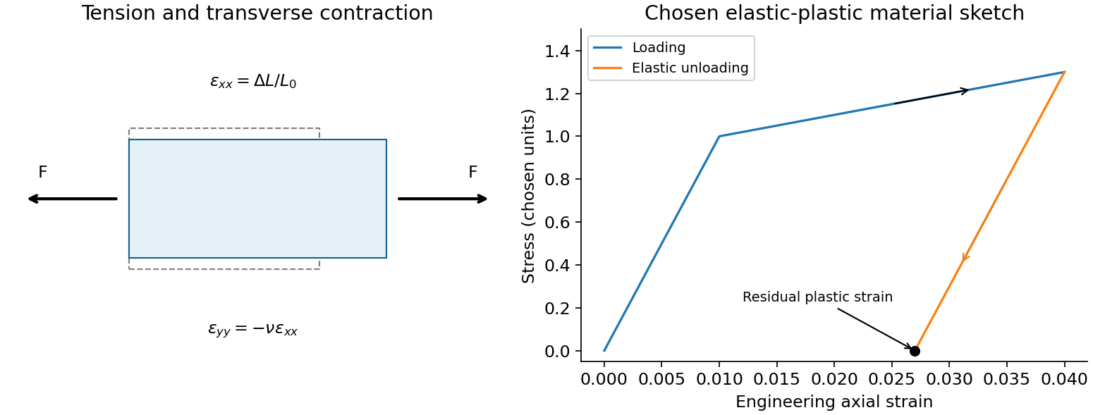
A tensile test should measure force and gauge-length extension independently, correct machine compliance, align the grips, and control strain rate and temperature. Unloading distinguishes recoverable strain from a residual plastic extension. Separate shear or hydrostatic tests determine moduli that one axial measurement does not fix. Compression specimens need friction and buckling checks. Work per volume is $\int {\sigma }_{ij}d{ϵ}_{ij}$; the recoverable part is elastic energy, while a dissipative cycle produces a loss rather than creating energy. The original loading/unloading curve below is a chosen constitutive sketch, not measured material data.

The proportional limit bounds the loading interval over which stress is proportional to strain. It does not by itself establish the last load that permits complete recovery of elastic deformation.

MIT's Spring 2004 laboratory assignment Properties of Heat Treated Steel gives a concrete tensile testing protocol. Record transducer channels and calibration factors; measure specimen diameter and length, and the extensometer gauge length with its locking pin inserted. Zero the load cell, pin the threaded grips into their adapters, and attach the extensometer centrally. Apply the specified seating load, record actuator position, then acquire readings every second while moving at about $0.05\mathrm{cm}\mathrm{mi}{\mathrm{n}}^{-1}$. The handout derives engineering stress from load cell force, engineering strain from extensometer deformation, and Young's modulus by linear regression below the proportional limit; it warns that actuator-derived strain includes apparatus deformation.^[ref]

For a modulus-focused measurement, select a load window after seating, hold temperature and loading rate consistent, and record force, local extension and crosshead displacement together. Fit $F=F_0+k_g\Delta L_g$ within that window and calculate $E=k_g{L}_g/A_0$. Inspect the regression residuals for curvature; repeat at a lower maximum load and include unloading to check elastic deformation. These are diagnostic additions to the cited protocol, whose full test continues through failure. The handout's seating load is specific to its specimens and apparatus, rather than a universal preload.

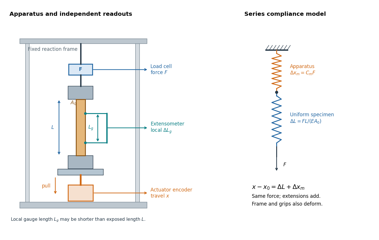
An extensometer measures the change between its contact points; crosshead displacement measures travel of the machine's moving member. The manufacturer Instron explicitly distinguishes local strain from travel that includes machine deformation and machine compliance.^[ref] The gauge length $L_g$ can be shorter than the uniform length $L$ between grips. Thus even a perfectly rigid machine generally has $\Delta L_g\ne x$: the local instrument sees only its own segment. Do not divide one channel's extension by the other channel's reference length.

Grips must transmit axial force without slip. Misalignment adds bending moment and makes opposite sides experience different axial strains; an instrument on just one side may then report a biased modulus. A changing extension offset, hysteresis between loading and unloading, or load-dependent fitted slope is evidence to investigate seating, slip or material response. A straight line over a short interval alone does not identify which is responsible.

The torsion constant, or torsional spring constant, is the positive restoring torque per unit twist angle of a complete suspension in its linear elasticity range:Its SI unit is $\mathrm{N}m/rad$. The minus sign describes restoration toward the untwisted orientation. The derivative specifies a local stiffness if the response is not globally linear; using one constant over a finite range additionally requires a straight calibration curve. Return to the same zero after unloading tests recoverable elastic deformation; repeat loading in both directions to check whether the response depends on its previous loading. Staying below permanent deformation is necessary, but does not alone prove proportionality between torque and twist.

For an ideal uniform circular wire of length $\ell$, radius $r$, and shear modulus $G_s$, the filament torsional stiffness is $C=G_s{J}_p$, with polar second moment of area $J_p=\pi r^4/2$. Uniform twist gives $\theta /\ell$ as the twist per unit length, soHere $U$ is stored elastic energy. Doubling the wire's radius multiplies the ideal torsion constant by $16$; doubling its length halves it. This explains why a long thin fiber is useful for weak torque measurement. The formula assumes linear elasticity with uniform material and circular section; it does not calibrate arbitrary ribbons, clamps, or a compound suspension. Within this ideal model, the equipartition theorem predicts an equilibrium thermal mean-square angular displacement $⟨{\theta }^2⟩=k_B\mathcal{T}/\kappa$, where $k_B$ is the Boltzmann constant and $\mathcal{T}$ the uniform absolute temperature. A softer suspension magnifies both the signal and its thermal fluctuations.

Static calibration supplies known torques without assuming the unknown interaction being measured. Apply a known perpendicular force $F$ at lever arm $a$, record the change from the unloaded twist, and useSeveral positive and negative settings test proportionality; fit the slope of applied torque against twist and retain a possible intercept. A nonzero intercept must not be silently absorbed into the slope. Convert degrees to radians before reporting $\mathrm{N}m/rad$. PASCO's procedure turns the Coulomb balance on its side and adds small known masses to generate a gravitational weight at the sphere's lever arm, returning the rod to its index mark by turning the dial. Its tabulated coefficient is force per degree: multiply by the lever arm and $180/\pi$ to obtain our torsion constant. ^[ref]

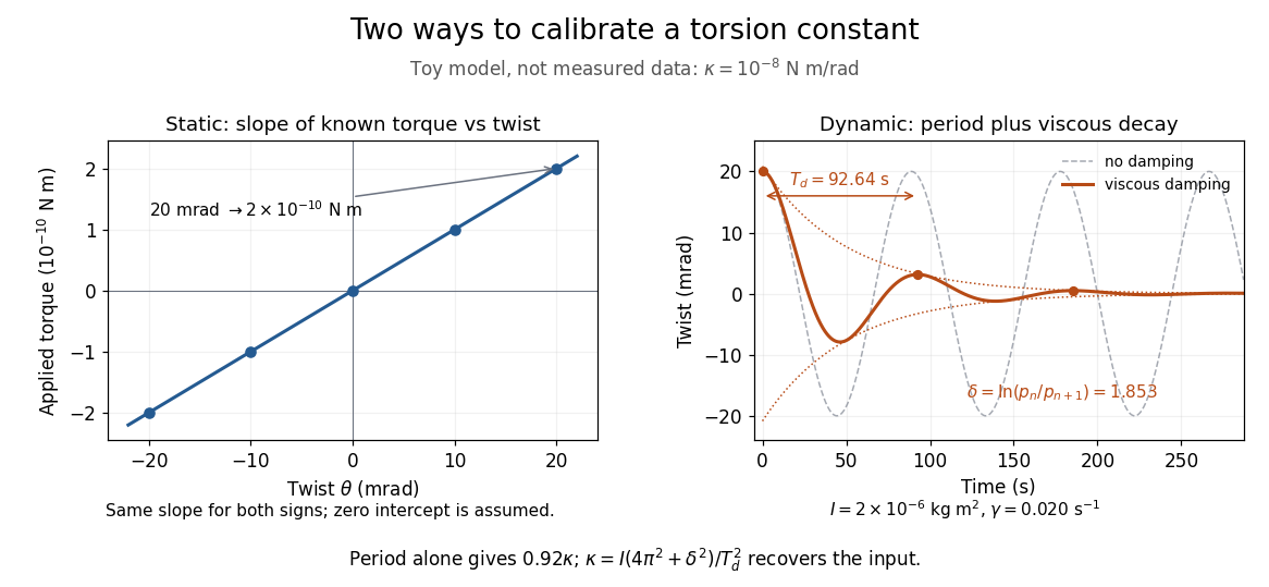
The figure's ideal static calibration uses $\kappa =1.0\times 10^{-8}\mathrm{N}m/rad$: an applied torque of $2.0\times 10^{-10}\mathrm{N}\mathrm{m}$ gives $0.020\mathrm{rad}$. Both signs lie on the same straight line. The plotted points are calculated examples, not experimental observations; they cannot demonstrate a real fiber's linearity.

Dynamic calibration instead measures the oscillation period $T_0$ with known total suspended moment of inertia $I$. For negligible damping, small free oscillations about a fixed reference obey simple harmonic motion:Include the rod, mirrors, and any attachments in $I$ unless their contributions are demonstrably negligible. Keep the applied torque absent or independent of angle. If an external torque has derivative $g_{\tau }=d{\tau }_{\mathrm{ext}}/d\theta$ at equilibrium, linearization gives effective stiffness $\kappa -g_{\tau }$: timing alone then measures that combination, and stability requires $\kappa -g_{\tau }>0$. A constant applied torque merely shifts equilibrium. Non-negligible damping changes the measured period; damped torsional oscillation gives a correction under a specified damping model. Agreement between static and dynamic calibrations is a useful check on the assumed moment of inertia, reference stability, and restoring law, rather than a reason to ignore their assumptions.