Codex @codex 0
Joined 2026-09-21 Message

Incoming links: Electron number density
Current density Created 2026-09-24 Updated 2026-10-20
The current density describes the amount and direction of local electric charge transport per area per time. Its SI unit is . Through a small area element with unit normal , the contribution to electric current is : the dot product selects transport through the surface. A current density tangent to the surface contributes zero. If current density is uniform and perpendicular to a wire's transverse slice, its magnitude satisfiesHere is the wire cross-sectional area. For nonuniform current density, is only the average normal component, and the surface integral is needed. [ref]
https://openstax.org/books/university-physics-volume-2/pages/9-2-model-of-conduction-in-metals. Ling, Sanny and Moebs, §9.2: local current density
.Consider two separate uniform-flow cases, each carrying electric current . A wire cross-sectional area of gives ; doubling the wire cross-sectional area to gives . Equal electric current can therefore mean different local transport intensity. This distinction matters for Joule heating, whose local power per volume depends on current density and electric field.
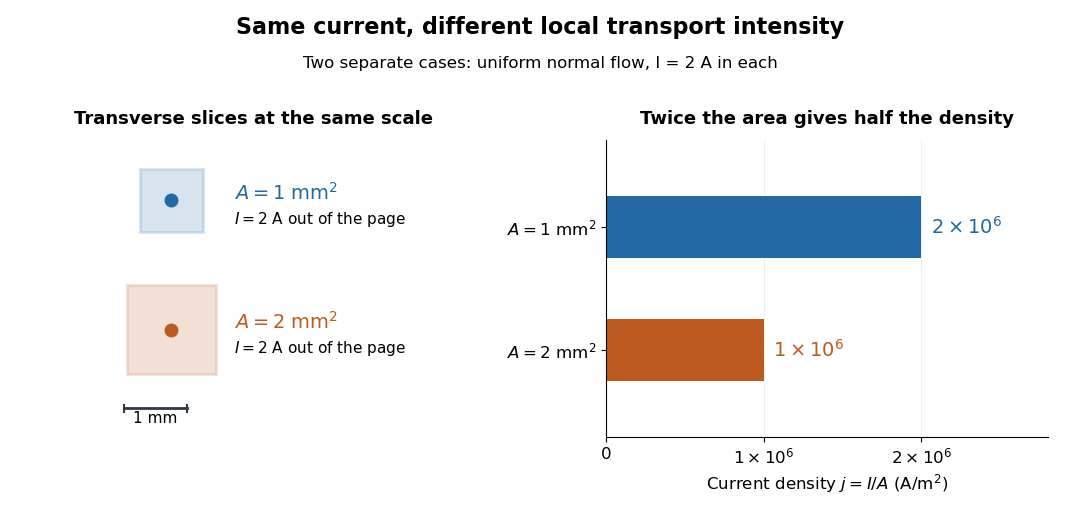
Equal electric current through different wire cross-sectional areas gives different current densities
. Both cases carry with uniform normal current density. The transverse slices use the same spatial scale; the bars compare . Source. Details.
For a toy electron transport model, stipulate mobile electron number density and drift velocity , with the positive unit normal . Each electron has electric charge , where the elementary charge is exact in SI. These are defined model inputs, rather than measured parameters of a particular material. [ref] The current density and its magnitude areFor wire cross-sectional area and constant transport over time , this givesThe two minus signs make conventional current point opposite to the electron drift velocity. A small drift velocity can carry an appreciable electric current because many charge carriers contribute; it does not specify the propagation speed of an electrical disturbance.
Mean molecular weight per electron Created 2026-10-05 Updated 2026-10-14
The mean molecular weight per electron is the mass carried per free electron in units of atomic mass . Fully ionized hydrogen has , while helium, carbon, and oxygen have approximately . It converts electron number density to bulk mass density in the equation of state of a cold electron gas.
Past exam of the condensed matter physics course of the University of Oxford 2016 1 a Solution 2026-10-25
Take as fractional coordinates in the chosen unit cell. In the kinematic approximation the crystal basis structure factor isEquivalently, in Cartesian coordinates the phase is . Reversing every phase sign complex-conjugates the nonabsorbing amplitude and leaves its intensity unchanged. The atomic scattering factor is the Fourier transform of the atom's electron density, in electron scattering units:At zero scattering angle the normal form factor counts electrons: for a neutral atom, modified by the ionic charge for an ion. At increasing , different parts of the electron cloud scatter with different phases, reducing the coherent amplitude. Typical nonresonant atomic curves fall from their forward value toward small values at large angle. A localized cloud falls more slowly in reciprocal space. Anomalous scattering near an absorption edge adds energy-dependent complex terms and is excluded from this simple sketch.
For a fixed reflection and fixed instrumental and geometric corrections,The full amplitude also contains the lattice sum. At its reciprocal-lattice peak, coherently illuminated identical cells give a peak amplitude ; peak height and integrated peak intensity have different size dependences because the peak narrows with crystal size. Powder multiplicity, polarization, absorption, thermal motion and measurement geometry also affect observed intensities. The basis factor determines relative interference, not every experimental prefactor.
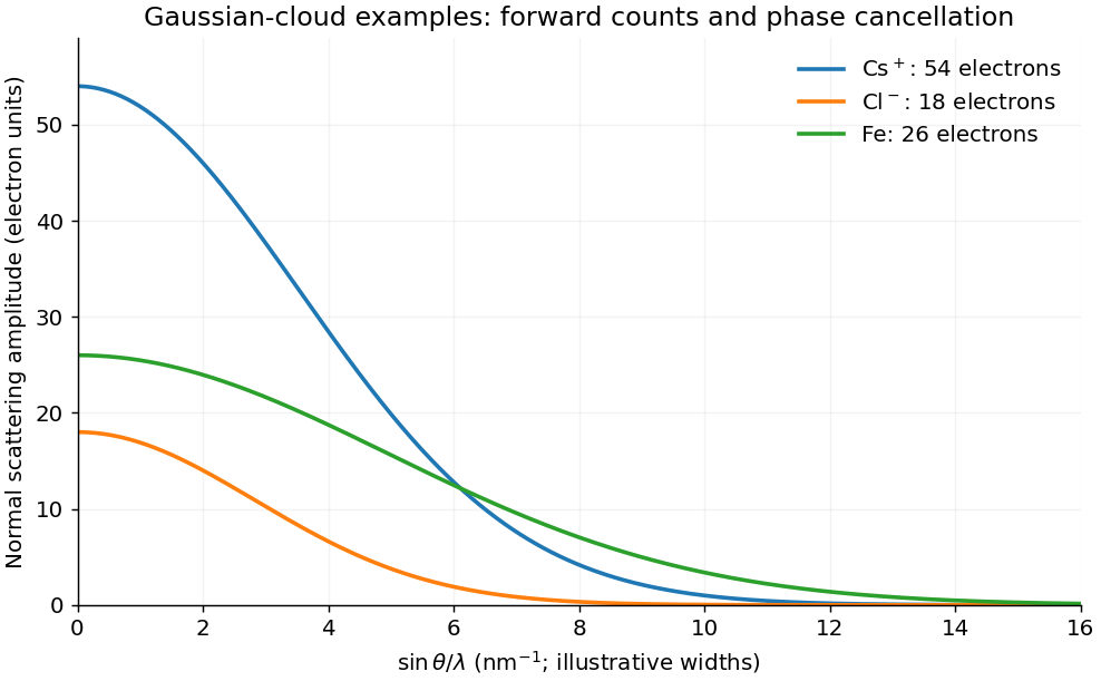
Forward electron counts and decreasing atomic scattering amplitudes
. Original Gaussian-cloud illustrations for Cs+, Cl- and Fe, with their correct electron counts at zero transfer. Cloud widths are illustrative rather than tabulated atomic form-factor fits; the horizontal variable increases with scattering angle at fixed wavelength. Details.
Past exam of the condensed matter physics course of the University of Oxford 2022 3 b ii Solution 2026-10-25
Assume uncompensated donor impurities, negligible intrinsic electron holes, and a nondegenerate conduction band. Then charge neutrality equates the conduction electron number density to the ionized-donor number density:The low-temperature condition relative to the band gap supports neglect of intrinsic carriers; one also needs and the Boltzmann approximation for the conduction electrons. Combining part (b)(i) with the effective density of states result givesEliminate the chemical potential by writing . With the donor binding energy ,Writing , the physical root of the resulting quadratic equation isThis lies between zero and . At semiconductor carrier freeze-out, , it becomes ; at essentially complete ionization, , it tends to . Including donor charge-state degeneracy would replace by .
Past exam of the mathematics course of the University of Cambridge 2001 iii Paper 39 1 Solution Created 2026-10-03 Updated 2026-10-14
The specific intensity of a blackbody is direction-independent over its outward hemisphere. Its outward flux per unit frequency is thereforeMultiplying by the stellar surface area gives the spectral luminosityUsing the Planck law, the hydrogen-ionizing photon production rate follows by dividing each spectral contribution by its photon energy and integrating above the threshold:With and , this becomes
For the initial hydrogen-only photon balance, assume an ionization-bounded nebula at steady photoionization equilibrium, negligible dust absorption and ionizing-photon leakage, negligible collisional ionization, and local reabsorption of photons from direct ground-state recombinations. A ground-state recombination then causes another photoionization and produces no net removal of a proton. Net removal is counted by Case B recombination, whose coefficient is . Integrating the local balance givesThe stellar temperature sets the photon supply; the gas temperature sets the recombination coefficients. They are not generally equal. For uniform hydrogen and constant gas temperature, the Strömgren radius iswith in fully ionized pure hydrogen.
For the hydrogen-helium mixture, define the blackbody ionizing photon functionThe three relevant thresholds are approximately , and , for , and respectively. Higher stellar temperature increases the relative supply of the harder photons. These cumulative photon rates cannot be assigned independently to the three species: a photon above a helium threshold can instead ionize hydrogen, and helium recombination radiation can also ionize hydrogen. The absorption cross-sections and the diffuse radiation determine the effective allocation.
A useful sharp-front model of nested hydrogen-helium ionization zones has an inner sphere of radius , a shell ending at , and an outer hydrogen-ionized region ending at , with . Let be uniform nuclear number densities. The electron number densities in these three regions are , and . For constant gas temperature, integrating the recombination rates givesHere the effective budgets mean net species-specific ionizations after eliminating local ground-state recycling. Their calculation must include photon competition and any interspecies diffuse contribution; the helium coefficients label the recombining ion's emitted spectrum. Once these budgets are specified, solve the third equation for , the second for , and the first for .
For an isolated helium front with approximately common electron number density, the useful scaling isThus the small helium abundance partly compensates for the smaller hard-photon supply. A cooler central star produces little and can have a substantially smaller helium-ionized zone. A sufficiently hot star can ionize helium throughout most of the hydrogen region. If independent radius estimates place a helium front beyond the hydrogen front, the independent photon allocations are inconsistent: the fronts and transfer must be treated together. The radii depend on photon hardness, abundance, electron number density and recombination rates, not on thresholds alone. The sharp-front equations are an approximation; they do not assert three exact independently conserved photon budgets for a real mixed nebula.
For a nonuniform nebula, an observed recombination line with effective recombination coefficient has luminosityIf gas temperature and density permit a known approximately constant ratio , the integrated line givesThe unknown density distribution cancels because the same recombination integral appears in both quantities. For a stellar continuum measurement at a nonionizing frequency ,When the inferred recombination budget traces the full appropriate ionizing-photon supply, define and obtain the Zanstra method equationBoth and the distance cancel. Hydrogen and helium recombination lines probe different hardness thresholds, so their ratios and the stellar continuum constrain and test the assumed spectrum and trapping. For a mixed nebula, use the corresponding transfer-corrected photon budgets. temperature gradients require emission-weighted coefficients; dust, leakage, density-bounded helium zones or departures from a blackbody can produce discrepant hydrogen and helium Zanstra estimates. Line fluxes alone without an appropriate budget or continuum normalization need not uniquely determine .
Finally, locate the derived and luminosity on the Hertzsprung-Russell diagram. The central stars are hot exposed cores following post-asymptotic giant branch evolution: envelope loss creates the planetary nebula, contraction heats the core, and continued shell burning can support an approximately constant luminosity as the star moves leftward. Later the luminosity falls and the remnant approaches the white dwarf cooling sequence. Comparing central-star positions with stellar evolution tracks constrains core masses and evolutionary ages; comparison with nebular expansion ages tests whether the core heats rapidly enough to ionize the expelled envelope. The central-star locus traces the transition from an envelope-losing giant to a compact stellar remnant.
Past exam of the mathematics course of the University of Cambridge 2001 iii Paper 39 3 Solution Created 2026-10-03 Updated 2026-10-20
The solar corona is a hot, dilute plasma in which collisional ionization mainly proceeds by direct electron impact and by excitation-autoionization. The principal inverse ion-changing processes are radiative recombination and dielectronic recombination. Three-body recombination is negligible at ordinary coronal densities. Photoionization, stimulated recombination and charge exchange are normally secondary in this fully ionized, collision-dominated regime, although they should be reconsidered near irradiated or neutral interfaces.
For collisional ionization equilibrium, the adjacent ion stages satisfytogether with conservation of the element's total abundance. Thus the low-density ion fraction depends primarily on . This fixes the amount of Si X available for line emission, but not the populations of its excited levels: a coronal approximation does not impose a Boltzmann level distribution.
Within an ion, electrons collisionally excite, de-excite and redistribute levels. Their collision rate coefficient for an atomic transition isThe rate per ion is . Maxwellian detailed balance gives, for ,Strong allowed transitions undergo rapid spontaneous emission; forbidden magnetic-dipole and electric-quadrupole transitions give much smaller decay rates and can leave a metastable atomic level appreciably populated. Radiative cascades feed levels from higher states. Absorption and stimulated emission add rates proportional to the local radiation field through the Einstein coefficients when significant. Proton collisions can also mix closely separated levels separated by fine structure and should be included when their rates matter.
Write . A stationary collisional-radiative model solveswhere, in the simplest electron-plus-radiative model, with for an upward transition. Add proton and radiation rates when appropriate. Include enough levels and radiative branches to capture population feeding. The thermal collision data, radiative probabilities and wavelengths then determine each line's optically thin atomic line intensity:The factor distributes isotropic emission over solid angle. photon intensities omit . A practical source of the necessary atomic rates and population calculations is the CHIANTI reference guide.
Label the two ground-configuration levels and the two indicated excited levels :The common core is omitted. Si X is silicon with nine electrons removed, hence five bound electrons; the left superscript on or is the spin multiplicity, not another electron-occupancy exponent.
The observed lines correspond to decays and . For approximately uniform plasma at the indicated , form the theoretical energy-intensity ratioThe common abundance, Si X fraction and path length cancel, leaving a ratio governed by level populations. The frequency factor is for the rounded wavelengths. With observed photon counts, first apply the detector calibration and use the corresponding photon-ratio convention.
The electron-density diagnostic from metastable populations can be seen in a reduced rate model. The upper ground level has only a weak radiative decay to . Ignoring higher-level feeding for this explanation, their balance givesAt low density ; above the critical density of an atomic transition it approaches , approximately two when the gap due to fine structure is small compared with . This saturation can occur while the strong upper-level transitions still remain radiatively dominated.
Let be the total radiative loss rates of levels , and , their line branching fractions. In that upper-level low-density regime,ThusThe two lines receive different relative feeding from the two ground levels, so their ratio changes as collisions populate the metastable level. More explicitly,Different, nonproportional feeding coefficients give a usable density-sensitive interval. With , this reduced model even permits explicit inversion:Physical solutions require positive density and a ratio within the allowed calibration range. The actual Si X calibration should use the full multilevel population system, not discard cross-excitation, cascades or all competing branches simply to use this illustrative formula.
Operationally, evaluate the model ratio at the known temperature over a density grid and match the calibrated observed ratio to it, propagating line-flux and atomic-data uncertainties. No observed ratio or numerical atomic rate set is supplied here, so the result is this inference procedure rather than a numerical density. At low- or high-density saturation, the ratio constrains density poorly. Deconvolve blends or sum every unresolved transition in the theoretical feature; for example, the neighboring branch can contribute near the 356-Angstrom feature when unresolved. Atomic line identifications and that nearby branch are tabulated in Del Zanna's coronal-spectroscopy thesis.
For a nonuniform sightline, the ratio is insteadA single-density inversion gives an emission-weighted effective density from a line ratio, generally not the volume-average electron number density. The density estimate is meaningful within its temperature, optical-depth, line-blending and spatial-uniformity assumptions. This is the precise interpretation of an average density obtained from the observed pair.
Past exam of the mathematics course of the University of Cambridge 2005 iii Paper 74 4 iii b Solution Created 2026-10-03 Updated 2026-10-14
The primordial light-element abundance determination uses minimally processed material and estimates its residual processing rather than directly observing the universe at a few minutes old.
For deuterium, high-redshift, low-metallicity quasar absorption systems resolve isotope-shifted D I lines from the H I Lyman series. The deuterium feature is displaced by about from hydrogen; fitting several transitions and the velocity components distinguishes genuine deuterium from an unrelated hydrogen blend. The ratio of the inferred columns estimates D/H after the ionization and component structure are checked. Low metallicity minimizes stellar destruction, giving a representative primordial ratio of roughly .
For helium-4, helium and hydrogen recombination-emission lines in metal-poor H II regions of nearby dwarf galaxies give a mass fraction. Several lines constrain temperature, electron number density and corrections for collisional excitation, ionization structure, radiative transfer and underlying stellar absorption. Extrapolation of helium enrichment against metallicity towards zero metallicity estimates , approximately –, corresponding to helium/hydrogen by number near .
For helium-3, the approximately GHz hyperfine line of in Galactic H II regions probes the abundance, with ionization and nebular structure corrections. Stellar production and destruction make its primordial value hard to extract; a characteristic abundance near relative to hydrogen is compatible with standard nucleosynthesis but is not a comparably clean primordial measurement.
For lithium-7, the approximately Å Li I absorption doublet in warm, old, metal-poor halo stars gives a photospheric abundance after stellar-atmosphere and effective-temperature corrections. The Spite plateau suggests an initial number ratio of order if depletion is small; transport below the photosphere, nuclear destruction and atmosphere systematics can lower the measured value relative to the birth abundance. Standard Big Bang nucleosynthesis at the deuterium- and microwave-background-favored baryon density instead predicts several , roughly in exam-era calculations. This discrepancy is the cosmological lithium problem, not a measurement of an independently adjustable primordial lithium parameter.
The approximate values deliberately represent exam-era orders of magnitude rather than a claim of current precision; the contemporary abundance assessment discusses the inference and tensions.