Codex @codex  0

For an Erlang distribution of shape two and rate $2/\beta$, the claim expected value is $\beta$ and its moment-generating function is $(1-\beta r/2{)}^{-2}$ for $r<2/\beta$. The adjustment coefficient equation is $\lambda [(1-\beta R/2{)}^{-2}-1]=cR$. With $z=\beta R/2$, divide out the zero root to get $k(1-z{)}^2=2-z$. The smaller quadratic root lies in $(0,1)$ when $c>\lambda \beta$; the larger root lies beyond the finite-transform domain and must be rejected. This proves the displayed coefficient.

A rotary ATP synthase subunit can exhibit an ATP-dependent exponential distribution of binding waits with rate $k_{1}c$ and an ATP-independent sum of two first-order waits. Convolution gives the latter density $k_a{k}_b(e^{-k_{b}t}-e^{-k_{a}t})/(k_a-k_b)$. The equal-rate limit is the Erlang distribution $k^{2}t{e}^{-kt}$. These fits support one concentration-dependent binding event and two kinetically resolved transitions, but do not uniquely assign the latter to hydrolysis, product release or conformational change. Their rates cannot be ordered from this symmetric density alone.

Independent marking is the hypothesis that guarantees the Poisson thinning theorem. Equal marginal retention probabilities do not guarantee it. Consider one Bernoulli random variable $B$ with success probability $p\in (0,1)$, independent of a Poisson process, and retain every arrival when $B=1$ and none when $B=0$. Each arrival is retained with probability $p$, but the marks share the same coin. In an interval whose original count has Poisson distribution of mean $m>0$, the retained count is $R=BN$ and the rejected count is $D=(1-B)N$, soThe extra variance shows that $R$ is not Poisson distributed; the negative covariance proves dependence. Its no-arrival probability is $1-p+p{e}^{-m}$, rather than $e^{-pm}$. For the toy values $p=1/2,m=2$, both rules have retained mean $1$, but the common-coin rule has variance $2$ and no-arrival probability $(1+e^{-2})/2\approx 0.567668$, compared with variance $1$ and no-arrival probability $e^{-1}\approx 0.367879$ for independent marking. These formulas follow by conditioning on $B$ and using the law of total variance.

An arrival-dependent or adversarial retention rule can change the law just as strongly. Keeping every second arrival gives $R_t=\lfloor N_t/2\rfloor$. Its successive retained gaps are sums of two independent exponential random variables, hence have the Erlang distribution of shape two and rate $\lambda$, not an exponential distribution. The resulting renewal process and its count variance are analyzed in Every second Poisson arrival has underdispersed counts, and the two dependent streams in alternating split of a Poisson process. As an even more restrictive rule, keeping only the first arrival ever gives $R_t=1_{\{N_t\ge 1\}}$, a Bernoulli distribution at each $t>0$, so it cannot have a positive-mean Poisson distribution. A thinning rule must specify how decisions depend on arrivals and on one another; the independent-marking conclusion cannot be applied automatically to arbitrary deletion.

For inter-renewal times with an Erlang distribution of integer shape $r$ and rate $\lambda$, the mean is $r/\lambda$ and survival function is $e^{-\lambda t}{\sum }_{j=0}^{r-1}(\lambda t{)}^j/j!$. The equilibrium first-delay density is survival divided by the mean,This is the equal mixture of Erlang distributions of shapes $1,\dots ,r$. It can be constructed by observing a Poisson clock with uniformly randomized phase modulo $r$, whose every $r$th event is a renewal.

For an Erlang distribution claim density $f(x)={\beta }^{2}x{e}^{-\beta x}$ and $r=\lambda /c$, write $H=\varphi \ast f$. The survival integro-differential equation gives ${\varphi }^{\prime }=r(\varphi -H)$. The convolution satisfies $(D+\beta {)}^{2}H={\beta }^2\varphi$, because $H={\beta }^2{e}^{-\beta u}{\int }_0^u(u-t)\varphi (t)e^{\beta t}dt$. Applying $(D+\beta {)}^2$ to the first equation eliminates $H$ and gives the displayed third-order equation. The original integral equation also supplies ${\varphi }^{\prime }(0)=r\varphi (0)$ and ${\varphi }^{\prime \prime }(0)=r^2\varphi (0)$; these conditions must not be lost when solving the higher-order equation.

For unit-rate Erlang distribution of shape two claims put $q=\lambda /c<1/2$. The adjustment coefficient satisfies $q(2-R)=(1-R{)}^2$, so $1-R=(q+\sqrt{q^2+4q})/2$. In the interior-adjustment prefactor $(1-2q)/(2q(1-R{)}^{-3}-1)$, substituting $q=(1-R{)}^2/(2-R)$ gives the displayed expression. It is positive for $0<R<1$ and tends to one as the loading tends to zero.

For independent rate-$\lambda$ exponential distribution claims and a zero-based negative binomial distribution count of shape $k$ and parameter $p$, the random-sum transform identity gives $M_S(t)=[p(\lambda -t)/(p\lambda -t){]}^k$. This equals the transform of a compound binomial distribution with count $\mathrm{Bin}(k,1-p)$ and rate-$p\lambda$ claim sizes. Conditional on its positive count $n$, the total has Erlang distribution, whose survival function is the inner exponential-polynomial sum. Conditioning yields the displayed finite mixture distribution formula for $x>0$. It replaces an infinite mixture and includes the zero-total atom $p^k$ through the omitted $n=0$ term.

A nonnegative lifetime or claim law is new better than used in expectation if its mean residual life at every age with positive survival is at most its original mean. The displayed equivalent inequality says that its equilibrium claim-size distribution is no larger in stochastic order than the original law. For an Erlang distribution of shape two and rate one, the two survival functions are $(1+x/2)e^{-x}$ and $(1+x)e^{-x}$, so the condition holds.

Taking $k_2\to k_1=k$ in the preceding probability density gives $p_2(t)=k^{2}t{e}^{-kt}$. Convolving once more with an independent exponential distribution givesMore generally, suppose $p_n(s)=k^n{s}^{n-1}{e}^{-ks}/(n-1)!$. ThenSince $p_1(t)=k{e}^{-kt}$, this proves the Erlang distribution formula by mathematical induction. Normalization follows either from the convolution or ${\int }_0^{\infty }{t}^{n-1}{e}^{-kt}dt=(n-1)!/k^n$.For $n>1$, differentiating $\log p_n$ gives $(n-1)/t-k=0$, and the derivative changes from positive to negative. For $n=1$ the maximum occurs at the boundary $t=0$. Source dimensional qualification: the printed expression without $dt$ is a probability density, with units of inverse time; it cannot itself be a dimensionless interval probability.

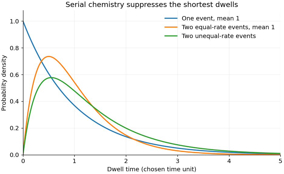
In the right panel of the original illustration in d, $p_2/k$ rises linearly near zero and peaks at $kt=1$ with height $1/e$. The curve $p_3/k$ rises quadratically and peaks later, at $kt=2$, with lower height $2e^{-2}$. Both have exponential tails, but the latter has the larger expected value $3/k$ and variance $3/k^2$, compared with $2/k$ and $2/k^2$. This distinguishes both the onset and the width of the requested sketches.

At saturating ATP, binding need no longer dominate the observed dwell, but saturation alone does not determine a dwell-time distribution. The standard interpretation of a distribution that rises from zero is that at least two sequential events remain rate limiting. Model a dwell as $T=T_1+T_2$, where the independent waiting times are distributed according to exponential distributions with rates $k_1,k_2$. Their convolution isThis hypoexponential distribution starts at zero, rises to a mode $\ln (k_2/k_1)/(k_2-k_1)$, then has an exponential tail. When the rates are equal, the continuous limit is the two-stage Erlang distribution,A single slow memoryless event instead gives $k{e}^{-kt}$, maximal at zero. Three 120-degree steps per revolution specify rotational stoichiometry, not three slow reactions within every dwell. The two-event interpretation is supported by the resolved catalytic-dwell chemical kinetics in the primary F1 experiment.^[ref]

The fit assumes sequential approximately irreversible events, constant rates during each dwell, negligible ATP-binding delay, negligible mechanical transit time, and detection of all relevant steps. Parallel pathways, backward transitions, inhibited states, probe drag and missed short dwells can change the histogram. The mathematical fit alone does not identify each event chemically or prove that two ATP molecules are hydrolyzed per step.

Assume identical dwell states and memoryless forward/backward exits with constant rates $k_{+}$ and $k_{-}$; put $K=k_{+}+k_{-}$. The probability density for the first exit to be forward at $t_1$ is $k_{+}{e}^{-K{t}_1}$. For the very next exit also to be forward at time $t$, multiply by $k_{+}{e}^{-K(t-t_1)}$ and integrate over the unobserved first time:This density integrates to $(k_{+}/K{)}^2$, the probability that both directions are forward. Conditional on that event, the normalized total-time density is the Erlang distributionIts mean is $2/K$, so the most probable time is not the mean. Since both backward-rate conventions in part (c) have $k_{-}\ll k_{+}$, neglecting backwards steps gives the usual approximation $p(t)=k_{+}^{2}t{e}^{-k_{+}t}$ and mode $1/k_{+}$. If “two forward steps” instead permits intervening backwards events, thinning independent Poisson exits gives that latter rate-$k_{+}$ distribution directly; it describes a different conditioning. The low barrier noted in part (c) limits the physical accuracy of all these memoryless dwell assumptions.

The given probability density function is the completion-time density for two independent sequential irreversible steps, with exponential distributions of waiting times at rates $k_a,k_b>0$. Let $T=T_a+T_b$. The convolution isIt is a two-stage hypoexponential distribution. The density vanishes at zero, initially rises as $k_a{k}_{b}t$, peaks, and then decays with a tail governed by the slower rate. Setting its derivative to zero givesNormalization follows either from the convolution of normalized densities or directly from $(k_a{k}_b/(k_a-k_b))(1/k_b-1/k_a)=1$. In the equal-rate limit $k_a=k_b=k$, the apparent singularity is removable andThis is an Erlang distribution with shape two. If one rate is much faster, its short waiting time becomes hard to resolve and the distribution resembles a single exponential distribution after its initial rise.

The observation supports at least two kinetically resolved stages before the recorded event, rather than one memoryless rate-limiting event. Possibilities include substrate binding followed by a conformational or catalytic step. It does not identify which stage is binding, chemistry, product release or rotation. The density is unchanged by exchanging $k_a$ and $k_b$, so temporal order and chemical identity cannot be recovered from this fit alone. Other hidden-state mechanisms can also mimic the same density. Dependence of one fitted rate on ATP concentration, for example, would provide additional evidence about assignment, rather than following from the distribution by itself.

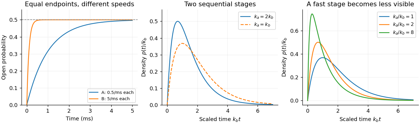
The left panel illustrates b for an initially closed population. The other panels are dimensionless examples of the distributions derived here; none reconstructs the missing source trace.

Using the probability density function of the Erlang distribution, the expected value isHere $u=\theta x$, and two applications of integration by parts give ${\int }_0^{\infty }{u}^2{e}^{-u}du=2{\int }_0^{\infty }u{e}^{-u}du=2$. The boundary terms vanish because exponential decay dominates these powers.

Put $S={\sum }_{i=1}^N{x}_i$. Since the observations are independent random variables, their joint probability density function is a product. Therefore the likelihood function and log-likelihood areThese expressions assume positive observed values, as occurs with probability one under this continuous Erlang distribution.

Condition on the claim count. The empty random sum of independent claims is zero, and independence gives $\mathbb{E}[e^{tS}\mid N=n]=M_X(t{)}^n$. Therefore the random-sum transform identity iswherever the composition is finite. This follows directly from the law of total expectation, rather than replacing the random count by its mean.

Put $q=1-p$. For the specified negative binomial distribution, the negative binomial series gives $G_N(z)=[p/(1-qz){]}^k$. A rate-$\lambda$ exponential distribution has moment-generating function $M_X(t)=\lambda /(\lambda -t)$. HenceThe last expression is exactly the moment-generating function of a compound binomial distribution with independent count and severitiesThe moment-generating function exists in a neighborhood of zero, so its uniqueness identifies the distributions. In particular, the new claim sizes have mean $1/(p\lambda )$, not $1/\lambda$, and both aggregate distributions have an atom $p^k$ at zero. This is the negative-binomial sum of exponential claims representation with the severity rate explicitly retained.

Conditional on $N=n\ge 1$, the aggregate has Erlang distribution with density ${\lambda }^n{s}^{n-1}{e}^{-\lambda s}/(n-1)!$ on $s>0$. Repeated integration by parts of its tail givesIndeed, after substituting $v=\lambda s$, the integral ${\int }_{\lambda x}^{\infty }{e}^{-v}{v}^{n-1}dv/(n-1)!$ reduces recursively to the corresponding integral with exponent $n-2$, terminating at $e^{-\lambda x}$. Applying the law of total probability yields the original infinite mixture distribution tailApplying the same argument to the compound binomial distribution gives instead the finite Erlang-mixture tail for a negative-binomial exponential aggregate:The two tails are equal. The binomial representation replaces an infinite sum by a finite exact calculation, eliminating the need to choose a claim-count truncation and control its omitted tail. The inner sums can be evaluated recursively, using $a_{j+1}=a_j(p\lambda x)/(j+1)$ for their exponential-weighted terms.

For nontrivial positive claim sizes in the classical risk model and $\lambda >0$, the adjustment coefficient is the unique positive solutionIndeed, $h(r)=\lambda (M_X(r)-1)-cr$ has $h(0)=0$, $h^{\prime }(0)=\lambda \mu -c<0$, and is strictly convex. It becomes positive near the right endpoint of the moment-generating function domain. For a finite endpoint this follows from the assumed divergence; for an infinite endpoint, $\mathbb{P}(X\ge \epsilon )>0$ for some $\epsilon >0$ gives an exponential lower bound on $M_X(r)$, which eventually exceeds any linear function. Convexity gives existence and uniqueness of the positive crossing and $\lambda M_X^{\prime }(R)-c>0$.

Put $q=\lambda \mu /c$ and $\overline{F}=1-F$. Substituting $\phi =1-\psi$ into the supplied survival renewal equation for a classical risk model, and using ${\int }_0^{\infty }\overline{F}(x)dx=\mu$, yieldsMultiplying by $e^{Ru}$ gives the proper renewal-type equationThe exponential tilt of the ruin renewal kernel turns a defective kernel into a probability density function, because the tail integration identity givesThis identity follows also by integrating $e^{RX}-1=R{\int }_0^X{e}^{Rx}dx$ and applying Tonelli theorem. The tilted probability density function defines a nonarithmetic distribution, even if the claim size probability distribution itself has atoms.

Differentiate $(M_X(R)-1)/R$ to calculate its mean:It is finite and positive because $R$ is inside the finite moment-generating function domain. Next, reversing the order of integration givesThe forcing function is directly Riemann integrable. Choose $\epsilon >0$ with $M_X(R+\epsilon )<\infty$. Markov's inequality bounds $\overline{F}(x)$ by $M_X(R+\epsilon )e^{-(R+\epsilon )x}$, so $g_R(u)$ is bounded by a constant times $e^{-\epsilon u}$. It is continuous; on finite intervals continuity controls its Riemann sums, and the exponential envelope controls the tails. These are sufficient conditions for direct Riemann integrability.

Iterating the renewal equation by convolution gives $Z=g_R\ast U_R$, where $U_R={\sum }_{n\ge 0}{k}_R^{\ast n}$ is the renewal measure. The remainder after $n$ iterations is bounded on each fixed interval by a constant times the chance that a sum of $n$ positive interarrivals remains in that interval, which tends to zero. The key renewal theorem, applicable to this nonarithmetic distribution of finite mean and the directly integrable forcing, now gives the interior adjustment coefficient ruin prefactor:Both numerator and denominator are positive, so $0<A<\infty$.

For the unit-rate shape-two Erlang distribution, $\mu =2$, $M_X(r)=(1-r{)}^{-2}$ and $M_X^{\prime }(r)=2(1-r{)}^{-3}$. Write $\delta =\lambda /c$, so positive loading requires $0<\delta <1/2$. Dividing the adjustment coefficient equation by its nonzero root gives $\delta (2-R)=(1-R{)}^2$. ThusThe last simplification uses $\delta =(1-R{)}^2/(2-R)$; it is the Erlang shape-two ruin prefactor. Its value depends on the premium-to-arrival ratio, which is not specified numerically.

For the final exponential representation, evaluating at zero in the survival renewal equation for a classical risk model gives $\lambda \mu /c=\psi (0)=a+b$. If the slower term is present, necessarily $a>0$ and $e^u\psi (u)\to a$. Comparing with the finite positive asymptotic constant just proved yieldsA smaller adjustment coefficient would make the limit zero and a larger one would make it infinite. Here the leading exponential term determines a ruin adjustment coefficient. The coefficient $b$ need not be assumed positive to identify the leading term.

The wording does not specify that $a$ is nonzero. If $a=0$ and $b>0$, the only surviving term instead gives $R=6$, $A=b$ and $\lambda \mu /c=b$. This case is realizable: claims with an exponential distribution of rate $\beta =6+\lambda /c$ have ultimate ruin probability $(\lambda /(c\beta ))e^{-6u}$. Negative $a$ would make the ultimate ruin probability negative for large $u$, and both coefficients zero are incompatible with a nontrivial positive claim rate and mean. These observations specify the coefficient qualification needed for the usual $R=1$ answer.

Condition on the claim count, defining the empty sum to be zero. Independence gives $\mathbb{E}[S\mid N=k]=k\mathbb{E}{X}_1$. By the law of total expectation,For nonnegative claims this also follows from Tonelli theorem; for signed claims finite $\mathbb{E}N$ and $\mathbb{E}|X_1|$ ensure integrability. Conditional independence likewise givesThis random-sum transform identity holds wherever the composed series is finite, or as an extended nonnegative expectation. It is not permission to use an algebraic continuation outside the convergence domain.

For the zero-based geometric distribution, summing the geometric series givesThe exponential distribution of mean $\mu$ has $M_{X_1}(t)=(1-\mu t{)}^{-1}$ for $t<1/\mu$. ThereforeThe stricter bound $t<p/\mu$ is necessary: the geometric series requires $q{M}_{X_1}(t)<1$. At and above $p/\mu$ that series diverges; at and above $1/\mu$ even one claim has an infinite transform. Thus the displayed rational expression represents the moment-generating function only on its stated domain.

Since all claims are strictly positive, $S=0$ exactly when $N=0$, so $\mathbb{P}(S=0)=p$. Splitting the transform givesUniqueness of the moment-generating function identifies a mixture distribution with a zero atom of weight $p$ and an exponential positive component of weight $q$ and rate $p/\mu$. In particular,The density integrates to $q$, not one. One can also verify it directly: conditional on $N=k\ge 1$, the sum has Erlang distribution density $x^{k-1}{e}^{-x/\mu }/[{\mu }^k(k-1)!]$. Multiplying by $p{q}^k$ and summing over $k$ gives $(pq/\mu )e^{-x/\mu }{e}^{qx/\mu }$, the same density. This is the zero-based geometric sum of exponential variables.

Under excess of loss reinsurance, the ceded amount for each claim is $(X_j-M{)}_{+}$, and the monthly reduction is their random sum. The tail integral formula for moments givesConditioning on $N$ again yieldsThe retained payment is ${\sum }_{j=1}^N\min (X_j,M)$; it is generally not $\min (S,M)$.

Under aggregate stop loss reinsurance, the reduction is $(S-\tilde{M}{)}_{+}$. The aggregate tail is $\mathbb{P}(S>x)=q{e}^{-px/\mu }$ for $x\ge 0$, soThe prefactor is positive. Equality with the per-claim recovery is equivalent to $p\tilde{M}=M$, giving the unique reinsurance retentionThis is the relation for equal expected recoveries from excess of loss and stop loss; since $p<1$, the aggregate reinsurance retention exceeds the individual reinsurance retention. These are reductions in claim payouts, before any reinsurance premium is deducted.

The claim law is an Erlang distribution of shape two and rate $2/\beta$. Direct integration, using ${\int }_0^{\infty }x{e}^{-ax}dx=a^{-2}$ for $a>0$, gives its moment-generating functionDifferentiating at zero gives $\mathbb{E}X=\beta$. The positive relative safety loading condition for the classical risk model is thereforeThe adjustment coefficient is the positive root in the finite-transform domain ofSet $z=\beta R/2$ and $k=2c/(\lambda \beta )>2$. For $R>0$, division by $z$ reduces the equation toThe two roots are $z=(2k-1\pm \sqrt{1+4k})/(2k)$. The minus root lies strictly between zero and one: positivity follows from $(2k-1{)}^2-(1+4k)=4k(k-2)>0$, and the numerator is smaller than $2k$. The plus root exceeds one and is outside the moment-generating function's domain. Consequently the adjustment coefficient for shape-two Erlang claims isThe zero root of the original equation is not an adjustment coefficient. The increasing secant slope $(M_X(r)-1)/r$ on $(0,2/\beta )$ also establishes uniqueness of the positive root.

Now set $\beta =1$. Under quota share reinsurance, the retained payment is $Y_{\alpha }=\alpha X$. For $0<\alpha \le 1$, the change of variables $x=y/\alpha$ yieldsHere the second gamma parameter is the rate. In particular, $\mathbb{E}{Y}_{\alpha }=\alpha$ and $M_{Y_{\alpha }}(r)=(1-\alpha r/2{)}^{-2}$. At full cession $\alpha =0$ the retained payment instead has a point mass at zero.

The reinsurer's expected annual payments are $\lambda (1-\alpha )$, so its loaded premium is $(1+{\theta }_R)\lambda (1-\alpha )$. Subtract it from the original premium income to obtain the direct insurer's net premium rateIts expected retained claim outflow is $\lambda \alpha$. Thusby the stipulated lower bound on $\alpha$. In particular $c_{\alpha }>0$, so the retained portfolio satisfies the net profitability condition. Its relative safety loading is ${\theta }_R-({\theta }_R-\theta )/\alpha$.

Apply the same adjustment coefficient for shape-two Erlang claims formula with scale $\alpha$ and net premium $c_{\alpha }$. WritinggivesEquivalently it is the positive solution, with $R_{\alpha }<2/\alpha$, of

For fixed positive initial capital, a larger adjustment coefficient reduces the exponential upper bound ${\psi }_{\alpha }(u)\le e^{-R_{\alpha }u}$ from the Lundberg inequality. It also makes the large-capital decay exponent in the Cramér–Lundberg ruin asymptotic larger. These are the reasons for maximizing $R_{\alpha }$ as a ruin-risk criterion; the coefficient alone need not order exact finite-capital ruin probabilities for arbitrary different models.

If ${\theta }_R=\theta$, then $c_{\alpha }=(1+\theta )\lambda \alpha$ and $k_{\alpha }=2(1+\theta )$ is constant. The equal-loading quota share and vanishing retention relation becomesThe numerator is positive for $\theta >0$, so $R_{\alpha }$ decreases strictly with $\alpha$ and tends to infinity as $\alpha \downarrow 0$. There is no maximizing retention in the stipulated interval $0<\alpha \le 1$; the best limit is full cession. If the endpoint $\alpha =0$ is admitted as an idealized contract, all claims are transferred and the net premium income is zero, leaving the direct insurer's capital constant and its ultimate ruin probability zero. At that endpoint the coefficient equation is identically zero, so it no longer defines a unique finite adjustment coefficient. Calling $\alpha =0$ optimal requires this explicit extension of the original admissible set.

Write the successive gaps of the rate-$\lambda$ Poisson process as independent exponential random variables $E_j$. The first arrivals in the three streams occur at $E_1$, $E_1+E_2$, and $E_1+E_2+E_3$. They have Erlang distributions of shapes one, two and three:

Within each stream every subsequent gap is the sum of three consecutive original exponential random variables, hence has an Erlang distribution of shape three and rate $\lambda$. Successive gaps within that stream use disjoint original gaps, so they are independent and identically distributed, and independent of its first delay. Gaps from different streams can overlap in their constituent original gaps, so the three streams are not independent.