Codex @codex  0

For a nonzero real function, write $\Lambda =F/G$ with $G={\int }_a^{b}w{y}^{2}dx>0$. Multiplying the Sturm-Liouville equation by $y$ and integrating givesThus the stated vanishing boundary product proves $\lambda =\Lambda [y]$.

For the variational statement, the first variation isWith admissible boundary conditions that also make $[p{y}^{\prime }\eta {]}_a^b=0$ for every allowed variation, the fundamental lemma of the calculus of variations identifies stationary functions with the eigenfunctions and stationary values with their eigenvalues. Zero Dirichlet boundary conditions, zero Neumann boundary conditions, and matched periodic data give familiar examples. The single printed condition $[py{y}^{\prime }{]}_a^b=0$ proves the quotient identity but, by itself, does not specify the admissible variations needed for stationarity; the boundary conditions for variational Rayleigh quotients make this distinction explicit.

For the half-line equation, multiplication by $x^{n-1}$ gives $p=w=x^{n-1}$ and $q=x^{n+1}$. Use the regular radial boundary condition at zero and square-integrable decay at infinity, under which the proposed Gaussian is admissible. With $y=e^{a{x}^2}$, $a<0$, $y^{\prime }=2axy$, soThe ratio of the two Gaussian integrals is $n/(-4a)$, from a change of variables and the Gamma function recurrence. Differentiating gives ${\Lambda }^{\prime }(a)=-n[1-1/(4a^2)]$, so the minimum on $a<0$ occurs at $a=-1/2$. The Gaussian variational bound for a radial harmonic oscillator therefore givesHere the trial actually satisfies the differential equation with $\lambda =n$. Moreover, on the same regular decaying domain, integration by parts gives $F[y]-nG[y]={\int }_0^{\infty }{x}^{n-1}(y^{\prime }+xy{)}^{2}dx\ge 0$. Hence the estimate is exact, with $\boxed{{\lambda }_0=n}$. For $n=1$, regular radial data mean the Neumann boundary condition $y^{\prime }(0)=0$; imposing a zero Dirichlet boundary condition there would exclude this trial and give a different problem.

For nonzero $y$ with $G[y]>0$, the first variation of the Rayleigh quotient under $y\mapsto y+\epsilon h$ isChoose fixed admissible homogeneous boundary conditions that make the variation boundary term vanish, such as zero endpoint values or zero endpoint derivatives. Compactly supported $h$ then show that a stationary function satisfies the Sturm-Liouville equation with $\lambda =\Lambda [y]$. Conversely an eigenfunction satisfying those admissible conditions makes the variation zero. Multiplying its differential equation by $y$ and integrating by parts givesso the stipulated energy boundary term yields $\Lambda [y]=\lambda$. The displayed energy condition alone is not a full specification of the admissible variations; it must be paired with boundary conditions for this variational equivalence.

For the final Dirichlet problem take the trial function $y=\sin x$, with $p=1,q=0,w=x$. ThenThe Rayleigh-Ritz variational principle makes this an upper bound for the lowest eigenvalue. It is strictly above the true value: equality would require $\sin x$ itself to be a lowest eigenfunction, but $y^{\prime \prime }+\lambda xy=(-1+\lambda x)\sin x$ cannot vanish throughout $(0,\pi )$ for a constant $\lambda$. ThereforeAlthough the weight vanishes at the left endpoint, it is positive in the interior and its weighted quadratic norm is positive for every nonzero admissible continuous function; this does not obstruct the stated Dirichlet variational comparison.

Take fixed-endpoint variations $y_{\epsilon }=y+\epsilon \eta$ with $\eta (a)=\eta (b)=0$. The first variation isThe boundary term vanishes by the endpoint conditions. The fundamental lemma of the calculus of variations gives the Euler-Lagrange equation $f_y-d(f_{y^{\prime }})/dx=0$. Along its solutions,When $f_x=0$, this proves the Beltrami identity $f-y^{\prime }{f}_{y^{\prime }}=\text{constant}$.

For the surface $z=F(y)$, the line element is $d{s}^2=d{x}^2+[1+F^{\prime }(y{)}^2]d{y}^2$. The arc-length integrand for a graph $y(x)$ is $\mathcal{L}=\sqrt{1+[1+F^{\prime }(y{)}^2]y^{\prime 2}}$. It has no explicit $x$ dependence and satisfies $\mathcal{L}-y^{\prime }{\mathcal{L}}_{y^{\prime }}=1/\mathcal{L}$. Thus $[1+F^{\prime }(y{)}^2]y^{\prime 2}$ is constant. Choosing the fixed direction along a smooth nonconstant segment and integrating yieldsThe same result follows by defining the transverse arc coordinate $u(y)={\int }^y\sqrt{1+F^{\prime }(s{)}^2}ds$, which changes the metric to $d{s}^2=d{x}^2+d{u}^2$. Its geodesics are straight lines in $(x,u)$ coordinates. This proves the formula for geodesics on a generalized cylinder and shows it gives locally shortest paths. The additional straight lines $x=\text{constant}$ in the unrolled plane are also geodesics, but cannot be represented as graphs $y(x)$. Classical differential-geometric statements assume the surface has sufficient smoothness; the arc-length coordinate itself only requires the displayed integral to be well defined.

Fermat principle states that the optical path length $\mathcal{S}=\int nds$, or equivalently travel time $\mathcal{S}/c_0$, is stationary under small variations of the ray with fixed endpoints. Stationarity need not mean a global minimum.

For a plane ray written as $y(x)$, use $\mathcal{S}[y]=\int F(x,y,y^{\prime })dx$, with $F=n(x,y)\sqrt{1+y^{\prime 2}}$. Its stationary paths obey the Euler-Lagrange equationIt follows by taking the first variation, integrating the term in $\delta y^{\prime }$ by parts, and using zero endpoint variations.

For fixed endpoint values, a stationary differentiable path obeys the Euler-Lagrange equationIt follows by taking the first variation of the functional and integrating the term in $\delta y^{\prime }$ by parts; $\delta y$ vanishes at the endpoints.

Choose homogeneous Dirichlet boundary conditions $\psi (a)=\psi (b)=0$, and take a nonzero real admissible trial $\psi$. Write the numerator as $F[\psi ]$ and denominator as $G[\psi ]>0$. For an endpoint-zero variation $\eta$, integration by parts givesThus the first variation of the Rayleigh quotient isBy the fundamental lemma of the calculus of variations, stationarity is equivalent toConversely, multiplying an eigenfunction equation by $\psi$ and integrating gives $F=\lambda G$, so its first variation vanishes. This establishes the equivalence for the chosen Sturm-Liouville problem. Homogeneous Neumann boundary conditions, or a mixed Dirichlet-Neumann pair, also cancel the boundary term; general Robin boundary conditions require adding the corresponding boundary contribution to the numerator.

The original PDF has a typographical omission: its displayed equation has $\lambda w(x)$ rather than $\lambda w(x)y(x)$ on the right. Taken literally, it is an inhomogeneous boundary value problem, not the stated Sturm-Liouville problem. The quotient and the later eigenfunction expansion identify the intended equation, which the following derivation produces explicitly.

Choose homogeneous Dirichlet boundary conditions $y(a)=y(b)=0$ and a nonzero real admissible $y$. Then $G[y]>0$ because $w>0$. For an endpoint-zero variation $\eta$, integration by parts givesThe first variation of the Rayleigh quotient is thusBy the fundamental lemma of the calculus of variations, stationarity is equivalent toConversely, multiply this corrected eigenvalue equation by $y$ and integrate. The same boundary cancellation gives $F[y]=\lambda G[y]$, so the first variation vanishes. This proves the requested equivalence for the intended equation. Homogeneous Neumann boundary conditions, or a Dirichlet condition at one end and a Neumann condition at the other, also eliminate the boundary term. General Robin boundary conditions would require the corresponding boundary contribution in the numerator.

For fixed initial and final coordinates, the two Euler-Lagrange equations areIndeed the first variation of the functional isIntegration by parts moves the time derivatives from the variations; their endpoint values are zero. The fundamental lemma of the calculus of variations then gives the two equations above.

The total derivative contributes only the boundary termThis is fixed by the endpoint data, so its first variation vanishes. It cannot change the Euler-Lagrange equations or which path minimizes $F$.

For a direct check, let $h=g_x\dot{x}+g_y\dot{y}$. ThenThe equality uses commuting mixed partial derivatives. Thus $\boxed{dg/dt\text{ contributes zero to both Euler-Lagrange equations}}$, as in total time derivatives preserve fixed-endpoint Euler-Lagrange equations.

This is an isoperimetric constraint, imposed on the whole path rather than separately at each time. Introduce a constant Lagrange multiplier $\lambda$ and replace the variational integrand by $\tilde{f}=f+\lambda u$. The modified Euler-Lagrange equations areSolve these together with the fixed endpoint conditions, treating $\lambda$ as an unknown constant, then choose its value so thatThe multiplier is constant because there is one scalar integral constraint. A condition imposed at every time would instead call for a time-dependent multiplier. As usual, this multiplier procedure assumes the constraint is regular, so its first variation does not vanish identically on all admissible variations.

Take nonzero real trial functions $y$ with $y,y^{\prime }$ square-integrable and sufficient decay for integration by parts. For a compactly supported variation $y\mapsto y+\epsilon \eta$, the first variations areThe quotient rule for the functional then yieldsBy the fundamental lemma of the calculus of variations, stationarity for all such $\eta$ is equivalent toConversely, multiplying a decaying eigenfunction equation by $y$ and using integration by parts gives $F[y]=EG[y]$, so its Rayleigh quotient equals $E$ and its first variation vanishes. Thus the stationary values of the functional are the energy eigenvalues. The word "extrema" in the question includes stationary points here: higher eigenfunctions can be saddle points of the unrestricted Rayleigh quotient.

The Rayleigh-Ritz variational principle givesChoose an admissible trial family, calculate its Rayleigh quotient, and minimize over its parameters to obtain the best upper bound within that family. Equality holds for the exact ground state; a restricted family generally gives only an upper bound.

Write $a(v,w)={\int }_{\Omega }a\nabla v\cdot \nabla w$ and $A[v]=a(v,v)$. The admissible set is the closed affine subspace $H_g^1=g+H_0^1$. Symmetry of the coefficient matrix givesIf $u$ minimizes the energy, its first variation vanishes: differentiating at $t=0$ gives $a(u,\phi )=0$. Hence $u$ is a weak solution.

Conversely, if $u$ is a weak solution, every admissible $v$ has $v-u\in H_0^1$ and thereforeby uniform ellipticity. This is the Dirichlet principle for the stated symmetric energy.

Let $\eta$ be a smooth variation with $\eta (a)=\eta (b)=0$. Assuming the usual continuous second derivatives of $F$, stationarity of the functional under $y+t\eta$ gives its first variationIntegration by parts removes the derivative of $\eta$; its boundary term vanishes because the endpoint values are fixed. Thusfor every such variation. The fundamental lemma of the calculus of variations implies the Euler-Lagrange equation $F_y=(d/dx)F_{y^{\prime }}$.

For arc length, $F=\sqrt{1+(y^{\prime }{)}^2}$, soThe function $s\mapsto s/\sqrt{1+s^2}$ is strictly increasing; hence $y^{\prime }$ is constant. With endpoints $(a,A)$ and $(b,B)$, $a<b$, the extremal isIt is also the global shortest curve: integrating the unit displacement vector dotted with the curve velocity gives the endpoint distance, which is at most the integrated speed by Cauchy-Schwarz inequality; the straight segment attains equality. A vertical segment is described parametrically or after rotating axes, since it cannot be represented by $y(x)$ on a nontrivial horizontal interval.

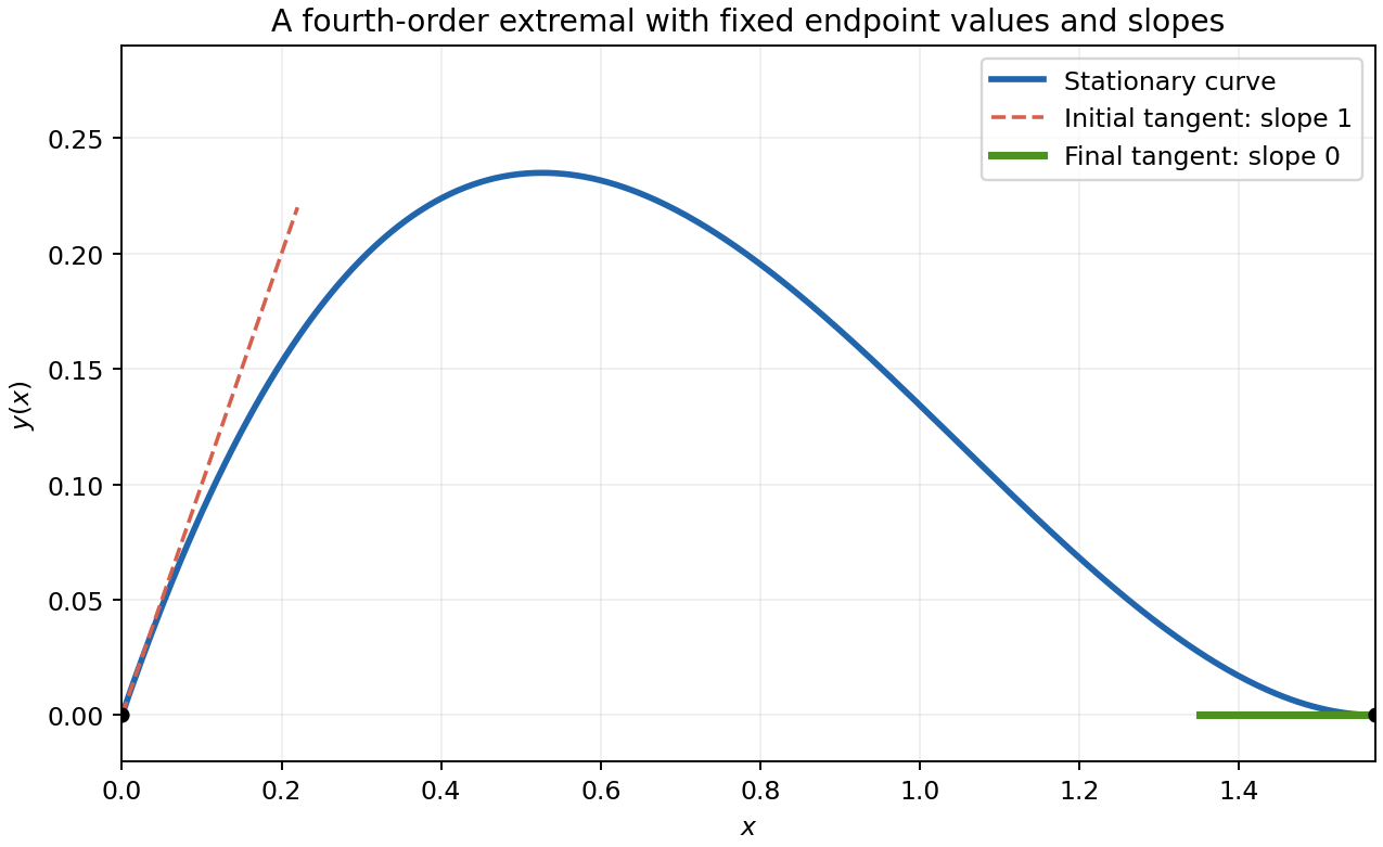
Let $y_{ϵ}=y+ϵ\eta$, with $\eta ={\eta }^{\prime }=0$ at both endpoints. At an extremal the first variation is zero:Integrate the second term by parts once and the third term twice. The boundary term isThe given fundamental lemma therefore givesThis is the classical form under the usual smoothness hypotheses ensuring the displayed derivatives exist; without that extra regularity the variation first yields its distributional form.

For the concrete functional the equation is $y^{(4)}-y=0$. Write $L=\pi /2$, $C=\cosh L$ and $S=\sinh L$. A general solution is $A\cos x+B\sin x+D\cosh x+E\sinh x$. The two initial conditions give $D=-A$ and $B+E=1$. The final derivative condition gives $A=EC/(1+S)$, and the final value condition then gives $E=(1+S)/2$. Thus an extremal isIt solves the differential equation, has initial value zero and initial derivative one, and at $L$ both its value and derivative vanish, using $C^2-S^2=1$. These checks verify all four prescribed endpoint conditions.

Take a smooth variation $u+\epsilon \eta$ with $\eta$ vanishing on the boundary; compactly supported test functions suffice for the interior equation. At an extremum, the first variation is zero:Integration by parts removes the derivatives from $\eta$. The boundary terms vanish, givingThe fundamental lemma of the calculus of variations gives the Euler-Lagrange equationThis is the classical equation for sufficiently smooth admissible extrema; for weaker regularity the first-variation identity supplies its weak form.

For the squared-gradient integrand, the equation is $2(u_{xx}+u_{yy}+u_{zz})=0$, namely the Laplace equation. Put $u_0=ax+by+cz$ and write any admissible function as $u=u_0+v$, with $v=0$ on the boundary. The energy identity isBy the divergence theorem, the middle integral is ${\int }_{\partial V}v(a,b,c)\cdot ndS=0$; equivalently it vanishes by weak integration by parts for zero-trace functions. The final term is nonnegative and vanishes at $v=0$. Thus this is a global minimum, not merely a stationary value:

Let $P=F_{y^{\prime }}$ and $Q=F_{y^{\prime \prime }}$. For a smooth variation $y+\epsilon \eta$, the first variation isHere the last expression follows by two integrations by parts. Taking variations supported in the interior and applying the fundamental lemma of the calculus of variations gives the Euler-Lagrange equation for a second-derivative functional:If both endpoint values and slopes are free, their independent variations force the natural boundary conditions for second-derivative functionalsIf an endpoint value or slope is fixed instead, its corresponding variation vanishes and the associated natural condition is not required.

For $H=y^{\prime \prime }Q-y^{\prime }(Q^{\prime }-P)-F$, differentiate using the chain rule:The Euler-Lagrange equation cancels the first term. Consequently $H^{\prime }=-F_x$, and if there is no explicit $x$ dependence,This is a Beltrami identity for a second-derivative functional.

Take independent smooth variations $y+\epsilon \eta$ and $z+\epsilon \zeta$. Differentiating the functional and using integration by parts gives its first variationFirst choose variations vanishing at the endpoints. To use the stated form of the fundamental lemma of the calculus of variations, take $\eta =(x-a)(b-x)\chi$ with arbitrary smooth $\chi$, and similarly for $\zeta$. The lemma makes $(x-a)(b-x)(F_y-d{F}_{y^{\prime }}/dx)$ vanish, and hence makes the unweighted coefficient vanish in the interior; continuity extends this to the endpoints. Applying the same argument to $z$ gives the Euler-Lagrange equationsIf either endpoint value of $y$ or $z$ is free, the corresponding variation there is arbitrary. The remaining boundary term gives the natural boundary conditions for a free endpoint: $F_{y^{\prime }}=0$ for a free $y$ value and $F_{z^{\prime }}=0$ for a free $z$ value at that endpoint. With both coordinates free at both endpoints, all four conditions apply.

For the specified integrand these equations reduce toand the natural conditions are $y^{\prime }=z^{\prime }=0$ at each free endpoint. Eliminating $z$ givesIts four independent modes give the full general solutionAt zero, $y^{\prime }(0)=C+2D$ and $z^{\prime }(0)=2C+D$. Vanishing forces $C=D=0$, givingAt $x=\pi /6$ the two derivative conditions become $A/2+\sqrt{3}B=0$ and $A+\sqrt{3}B/2=0$. Their coefficient determinant is nonzero, so $A=B=0$. Thus the unique stationary extremal with all four natural boundary conditions is $y=z=0$. The word extremal here means a stationary point of the functional; the indefinite integrand does not require this point to be a minimum.

Write $I[y]={\int }_a^{b}G(x,y,y^{\prime })dx$. For endpoint-zero variations $\eta$, the first variations areFor a normal constrained extremal, choose a variation ${\eta }_0$ with $\delta I({\eta }_0)\ne 0$. Given any $\eta$, use the implicit function theorem to choose a small correction in the ${\eta }_0$ direction so that $y+t\eta +s(t){\eta }_0$ preserves the constraint. Differentiating it and the stationarity condition at zero givesIntegrate the derivative-of-variation term by parts. Since the variations vanish at both endpoints, the boundary term is zero. The fundamental lemma of the calculus of variations then givesThe regularity condition on the constraint is what permits the coefficient of $F$ to be normalized to 1. In a degenerate case, the general multiplier statement uses ${\lambda }_{0}F-{\lambda }_{1}G$ with the two coefficients not both zero; the source's displayed form is the normal case.

For a string described as a function graph $r(x)=(x,y(x))$, its arc-length element is $|r^{\prime }(x)|dx=\sqrt{1+y^{\prime }(x{)}^2}dx$. Inextensibility therefore givesThis also forces $l\ge 2a$, with equality only for the straight function graph.

Write $K[y]={\int }_a^{b}G(x,y,y^{\prime })dx$. At a regular constrained extremal, the first variation of $K$ is not identically zero. Choose a variation $\zeta$ for which $\delta K[\zeta ]\ne 0$; the implicit function theorem supplies a correction in the $\zeta$ direction to each other variation so that $K$ remains one. Stationarity of $J$ on these corrected variations implies $\delta J=\lambda \delta K$ for one scalar $\lambda$.

Put $L=F-\lambda G$. Integration by parts gives, for an arbitrary twice continuously differentiable variation $\eta$,Taking variations with zero endpoint values and using the stated fundamental lemma of the calculus of variations gives the Euler-Lagrange equation. The remaining endpoint values are free and independent, giving the natural boundary conditions:If the constraint is not regular, the general multiplier statement permits an abnormal pair ${\lambda }_{0}F-{\lambda }_{1}G$ with ${\lambda }_0=0$; the source's general normal-form derivation implicitly excludes that case. In its quadratic example, regularity follows automatically from normalization: $\delta K[y]=2\int w{y}^2=2$.

For that example $L=p{y}^{\prime 2}-q{y}^2-\lambda w{y}^2$, so the equation and endpoint conditions reduce toMultiply the equation by $y$ and integrate. The boundary term $[p{y}^{\prime }y{]}_a^b$ vanishes, givingThe last integral equals one, so $\lambda =J[y]$, the functional value at the constrained extremal.

Finally multiply the equation for $y_1$ by $y_2$ and the equation for $y_2$ by $y_1$, then subtract and integrate. The derivative terms give only the vanishing boundary term $[p(y_2{y}_1^{\prime }-y_1{y}_2^{\prime }){]}_a^b$, while the $q$ terms cancel. Therefore $({\lambda }_1-{\lambda }_2){\int }_a^{b}w{y}_1{y}_{2}dx=0$. For distinct multipliers this proves

For the regular Sturm-Liouville setting assume $p$ is positive and continuously differentiable, $q,w$ are continuous, and $w>0$. Apply a multiplier to $J[y]-\lambda ({\int }_a^{b}w{y}^2-1)$. Its first variation, divided by two, isEndpoint-vanishing variations and the allowed fundamental lemma giveIf an endpoint value is free, its variation is arbitrary, giving the natural condition $p{y}^{\prime }=0$ at that endpoint. At a prescribed endpoint value the variation vanishes there, so no additional natural condition is imposed.

For eigenfunctions $u,v$ with different eigenvalues, multiply their equations by $v,u$ and subtract after integration. The resulting boundary expression $[p(u{v}^{\prime }-u^{\prime }v){]}_a^b$ vanishes under common homogeneous Dirichlet or common natural boundary conditions. Hence $({\lambda }_u-{\lambda }_v){\int }_a^{b}wuv=0$, proving weighted orthogonality.

For the final Dirichlet problem the normalized stationary modes areSolving $y^{\prime \prime }+(\lambda +1)y=0$ with both endpoint values zero gives these and excludes nonpositive $\lambda +1$. Distinct sine modes have zero integral product on $[0,1]$. Their Dirichlet values also make the same boundary expression vanish, which explains orthogonality even though their endpoint derivatives do not obey the natural conditions.

For global minimality, the Fourier sine expansion of an endpoint-vanishing function and Parseval's identities give $\int y^{\prime 2}=\sum k^2{\pi }^2{a}_k^2\ge {\pi }^2\sum a_k^2={\pi }^2\int y^2$. Equality holds exactly in the first sine eigenspace. ThereforeDistinct modes are orthogonal; the two sign choices of the same minimum are not orthogonal to each other. This distinguishes the family of stationary modes from the two representatives of the minimizing eigenspace in the question's wording.