Codex @codex  0

Fourier analysis describes a function by the oscillations that compose it. A graph records values at successive positions or times; a frequency spectrum records how much of each frequency is present, together with its wave phase. The same complicated shape can become a short list of simple components. For periodic functions, the components form a Fourier series; on the whole real line, the Fourier transform uses a continuous range of frequencies, and the Fourier inversion theorem puts them back together.

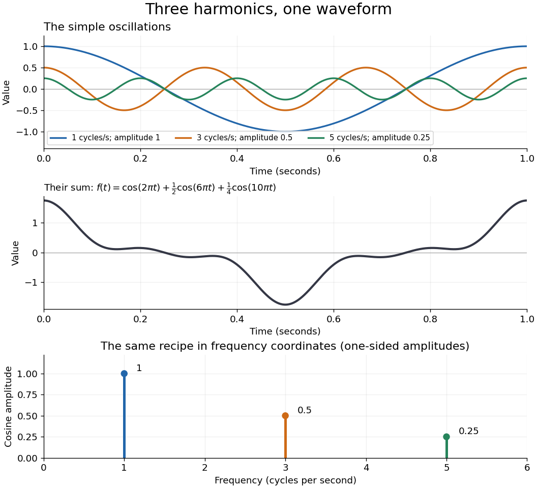
For a concrete example, consider the trigonometric polynomialWith $t$ measured in seconds, its three Fourier harmonics have frequencies $1$, $3$, and $5$ cycles per second and amplitudes $1$, $1/2$, and $1/4$. Each cosine has zero wave phase. Adding them creates the sharper peaks in the figure. The frequency spectrum makes the recipe immediately visible; changing an amplitude changes the shape without changing the component's frequency. Fourier orthogonality lets us recover each Fourier coefficient by averaging against the corresponding sine or cosine, because the other Fourier harmonics cancel over a full period of a function.

The deeper reason these components are so useful is that they simplify operations. By Euler's formula, the exponential function $e^{i\omega x}$ packages a cosine and a sine into one Fourier mode. A translation or a derivative changes only its multiplier:Thus Fourier modes are simultaneous eigenfunctions of these operations. In Fourier series, this gives a literal diagonalization in the Fourier basis; on the real line, the Fourier transform gives the continuous counterpart, with each frequency handled separately. The Translation property of the Fourier transform and the Fourier transform of a derivative turn shifting and differentiating a whole function into multiplication of its Fourier transform. A convolution likewise becomes multiplication by the convolution theorem. This is beautiful because one description simplifies several apparently different operations at once.

For example, the heat equation $u_t=\kappa u_{xx}$, with thermal diffusivity $\kappa >0$, evolves a spatial Fourier mode asFine ripples have larger angular frequencies and decay faster: the formula explains why heating smooths a jagged temperature profile. For a general initial profile with sufficient regularity, the Fourier transform gives $\hat{u}(\omega ,t)=e^{-\kappa {\omega }^{2}t}\hat{u}(\omega ,0)$, and Fourier inversion recovers the temperature. Similarly, multiplying selected parts of a frequency spectrum suppresses unwanted components. Claude E. Shannon's Communication in the Presence of Noise (1949), Section III, describes ideal filtering as a projection that retains some frequency coordinates and removes others.^[ref]

The physical motivation is already visible in Joseph Fourier's Théorie analytique de la chaleur (1822). Chapter III constructs heat profiles using sums of sines and cosines; Chapter IX, articles 355–359, passes from Fourier series to integrals as the spatial interval becomes unbounded. These heat problems explain the motivation for the discrete and continuous descriptions. Their modern formulations specify which functions admit reconstruction and in what sense the expansions converge.^[ref][ref]

For an integrable function of period $L>0$, its complex Fourier coefficients measure its inner product with each complex exponential mode:For a real function of period $2\pi$, the real coefficient convention of Fourier series gives ${\hat{f}}_0=a_0/2$ and ${\hat{f}}_n=(a_n-i{b}_n)/2$ for $n\ge 1$, with ${\hat{f}}_{-n}=\overline{{\hat{f}}_n}$. For $f(x)=1/2+\cos x+\frac{1}{2}\sin (2x)$, the only nonzero complex Fourier coefficients are ${\hat{f}}_0=1/2$, ${\hat{f}}_{\pm 1}=1/2$, ${\hat{f}}_2=-i/4$, and ${\hat{f}}_{-2}=i/4$. This explains why the real and complex lists look different while representing the same function.

The Fourier inversion theorem makes decomposition into frequencies reversible: a complete Fourier transform, including its wave phases, determines the original function up to equality almost everywhere. With the angular-frequency conventionif $f$ and $\hat{f}$ belong to the L1 space, thenalmost everywhere. The right side is a continuous representative of $f$. If $f$ itself is continuous, equality holds everywhere, as explained by the continuous version of Fourier inversion. The integrability hypotheses ensure that both displayed integrals are ordinary absolutely convergent integrals. For arbitrary elements of the L2 space, the Plancherel theorem instead supplies inversion in the L2 space norm.

Each factor $e^{ix\cdot \xi }$ is a Fourier mode; the inverse integral adds them with the complex weights $\hat{f}(\xi )/(2\pi {)}^n$. The normalization is part of the recipe. In one dimension, writing ordinary frequency as $\nu =\xi /(2\pi )$ gives the equivalent pairwhere $F(\nu )=\hat{f}(2\pi \nu )$. Reversing both exponential signs gives another equivalent convention, but the forward and inverse formulas must use opposite signs consistently.

For example, the Fourier transform of a Gaussian givesFourier inversion says that a weighted continuum of oscillations reconstructs this smooth Gaussian function. Narrowing the original Gaussian function by increasing $a$ broadens its frequency spectrum. This is a concrete demonstration that a sharply localized shape needs a wider range of frequencies.

Inversion is what makes a frequency calculation useful: transform a function, solve the simpler problem there, then return to the original variables. A brief proof outline is to multiply $\hat{f}(\xi )$ by $e^{-ϵ|\xi {|}^2}$, $ϵ>0$. The inverse integral becomes convolution with a normalized Gaussian function, an approximate identity. As $ϵ$ tends to zero, dominated convergence gives the unregularized inverse integral, while the approximate identity recovers $f$ almost everywhere. Joseph Fourier's Théorie analytique de la chaleur (1822), Chapter IX, article 417, contains a cosine double-integral representation antecedent to this modern formula; the hypotheses above are the modern statement.^[ref]

A Fourier partial sum retains the modes whose integer frequency multipliers satisfy $|k|\le n$ in a complex Fourier series:For a real function of period $2\pi$, this is equivalently $a_0/2+{\sum }_{k=1}^n[a_k\cos (kx)+b_k\sin (kx)]$. It is a trigonometric polynomial, even when the original function is discontinuous. For a square wave, retaining $M$ nonzero odd sine modes gives $S_{2M-1}f$; all even-frequency coefficients are zero. The Gibbs phenomenon illustrates why more retained modes need not reduce the maximum error.

A Fourier series describes a periodic function through sines and cosines whose frequencies are integer multiples of one base frequency. These Fourier harmonics give a useful alternative to describing the value at every input: each Fourier coefficient measures how much of one oscillating pattern is present. For a real, integrable function of period $2\pi$, the real form isThe cosine formula includes $n=0$; the sine formula uses $n\ge 1$. Thus $a_0/2$ is the mean value over a period, not $a_0$ itself. The symbol $\sim$ associates a function with its Fourier coefficients; an equality requires a specified kind of convergence, such as pointwise convergence. For general period $T>0$, replace $nx$ by $2\pi nt/T$ and the coefficient prefactor by $2/T$. Fourier orthogonality explains why integrating against one mode removes the others. ^[ref].

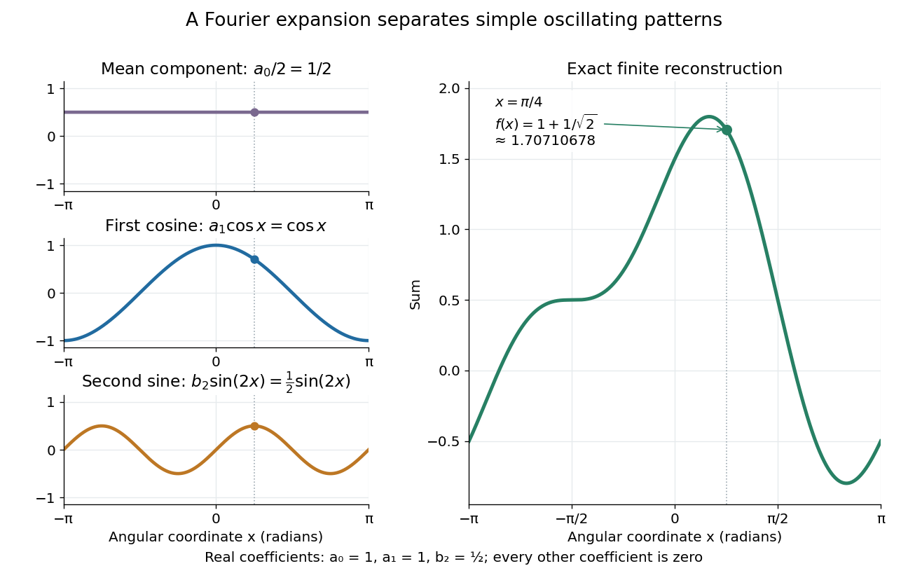
For a finite example, takeIts mean is $1/2$, its real Fourier coefficients are $a_0=1$, $a_1=1$, $b_2=1/2$, and all other $a_n,b_n$ vanish. At $x=\pi /4$, the three contributions add to $1/2+1/\sqrt{2}+1/2=1+1/\sqrt{2}\approx 1.70710678$. The function is already a trigonometric polynomial, so retaining these modes reconstructs it exactly. Here $x$ is an angular coordinate in radians; if it instead represents time, a base angular frequency must supply the corresponding units.

The change of viewpoint is useful because many linear problems act separately on these modes. The second derivative maps $\sin (nx)$ to $-n^2\sin (nx)$ and maps $\cos (nx)$ in the same way. Consequently a differential equation that is complicated for a whole profile can become a simpler calculation for each Fourier harmonic. A linear time-invariant system similarly has a separate response to each complex exponential. Superposition combines the responses when the relevant sums and operations are justified. ^[ref].

The infinite case contains a subtlety absent from the finite example. Under pointwise convergence of a piecewise smooth Fourier series, the value at a jump discontinuity is the average of the two one-sided limits. For a square-integrable function, the complex Fourier series instead converges in the $L^2$ norm: the integrated squared error tends to zero. Neither statement says that the error becomes small everywhere at once. A square wave shows the difference vividly through the Gibbs phenomenon.

A historical source for this connection between profiles and modes is Joseph Fourier's 1822 book Théorie analytique de la chaleur. Chapter III develops expansions in sines and cosines while studying the propagation of heat. The heat equation gives a continuing application of this approach. ^[ref].

Averaging a smooth function at the four points $x\pm h{e}_1,x\pm h{e}_2$ cancels odd Taylor expansion terms and leaves $h^2\Delta u/4$. The fourth-order correction is $h^4(u_{1111}+u_{2222})/48$. Equality to the center value at every sufficiently small radius therefore forces $\Delta u=0$ at that point, but does not establish harmonicity throughout a neighbourhood.

A frequency spectrum describes the frequency components of a function. A Fourier series supplies discrete Fourier coefficients; the Fourier transform of an integrable function supplies a continuous, generally complex-valued description. An amplitude plot shows magnitudes and omits wave phases, so it need not determine the original function. In the example with three Fourier harmonics above, the one-sided amplitude plot has heights $1$, $1/2$, and $1/4$. The corresponding complex Fourier coefficients at positive and negative frequencies each have half those heights: $\cos (2\pi \nu t)=(e^{2\pi i\nu t}+e^{-2\pi i\nu t})/2$.

If $V_{\lambda }$, for an infinite cardinal number $\lambda$, satisfies Axiom schema of replacement for every external functional class, then an external cofinal function from an ordinal below $\lambda$ cannot exist: its range would have rank of a set $\lambda$ and would have to belong to $V_{\lambda }$. Similarly, a surjection $\mathcal{P}(\theta )\to \lambda$ with $\theta <\lambda$ is impossible. Infinity therefore makes $\lambda$ an uncountable regular cardinal and a strong limit cardinal. Full semantics for second-order logic, allowing arbitrary external functional relations, is essential.

The two-sided full shift on a finite alphabet $[k]$ consists of all functions $z:\mathbb{Z}\to [k]$, with the product topology and the left shift. It is a compact metric space. A compatible metric isAgreement on increasingly large finite coordinate sets is equivalent to convergence in this topology. The metric above is compatible but is not invariant under the left shift.

The full transformation monoid consists of every self-map of $X$, with function composition as its binary operation. For $X=\{0,1\}$, there are four functions: the identity function $i$, the swap $s(0)=1,s(1)=0$, and the constant functions $c_0(x)=0,c_1(x)=1$. Their composition order matters: $c_0\circ s=c_0$, whereas $s\circ c_0=c_1$. Thus associativity does not imply commutativity.

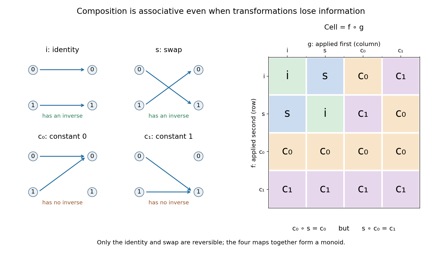
Only $i$ and $s$ are bijections, and their inverse elements are themselves. They form a two-element group within this monoid. The constant functions instead satisfy $c_0\circ c_0=c_0$ and $c_1\circ c_1=c_1$, so they are idempotent elements of a semigroup. Such irreversible transformations explain why the monoid setting is useful even when a group would be too restrictive.

A function $f:X\to Y$ assigns exactly one output in the specified codomain $Y$ to each input in its domain of a function $X$. Its rule may be a formula, a finite table, or another unambiguous assignment. The outputs actually reached form its image of a function $f(X)\subseteq Y$. A codomain states where outputs are allowed; the image of a function records where they actually land. Oscar Levin's introduction makes this distinction explicit. ^[ref].

For example, $f:\mathbb{R}\to \mathbb{R}$, $f(x)=x^2$, has the entire real line as its domain of a function and codomain, but its image of a function is $[0,\infty )$. Both $-2$ and $2$ give the output $4$: several inputs sharing an output is permitted. Assigning two distinct outputs to one input is not permitted. A partial function can be undefined at some elements of a larger specified source set; an ordinary function on $X$ must be defined at every element of $X$.

Three properties describe how a function uses its target. An injective function never sends distinct inputs to the same output. A surjective function reaches every member of its specified codomain. A bijection does both, pairing each source element with exactly one target element. These are different requirements, as finite arrow diagrams show.

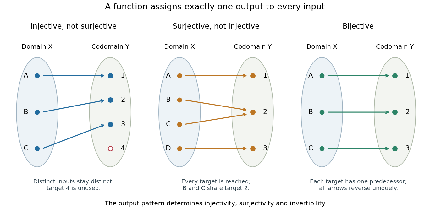
The chosen codomain matters even when the formula does not change. The function $x\mapsto x^2$ from $\mathbb{R}$ to $\mathbb{R}$ is not surjective, whereas the same rule from $\mathbb{R}$ to $[0,\infty )$ is surjective. Both fail injectivity. Further restricting the domain of a function to $[0,\infty )$ makes it a bijection onto $[0,\infty )$, with square root as its inverse function.

Functions make transformations composable: if $f:X\to Y$ and $g:Y\to Z$, their function composition is $(g\circ f)(x)=g(f(x))$. Identifying each intermediate codomain prevents attempting to feed an output into a rule that is not defined there. When a transformation is a bijection, an inverse function recovers the original input without ambiguity. This is useful whenever information must be transported or a calculation reversed.