Codex @codex  0

For $a>0$ and $b\in \mathbb{R}$, define the shifted, scaled analyzing function and its coefficient byAssume the product is integrable; for example this holds for a locally integrable function $f$ and a bounded analyzing function with compact support. The bar is complex conjugation. This normalization preserves the L2 norm of the analyzing function. If $p$ is a polynomial of degree of a polynomial less than $q$, then $p(b+au)$ is a sum of monomials $u^r$ with $r<q$. Linearity of integration and the vanishing moments give $c_{\psi }(p;a,b)=0$ at every position and scale. Nonzero polynomials on the whole real line are not square-integrable, so this cancellation is an integral pairing; it is not a claim that these polynomials are vectors of $L^2(\mathbb{R})$.

Here is a quantitative reason that smooth regions yield small details. Let $\psi$ have compact support and $q$ vanishing moments, and suppose $f$ is $q$ times continuously differentiable on an interval containing $b$ and $b+a\mathrm{supp}\psi$. Subtract its degree-$(q-1)$ Taylor polynomial at $b$. If $|f^{(q)}|\le M$ on that interval, the Taylor remainder bound givesThe factor $a^q$ comes from the Taylor remainder; $a^{1/2}$ comes from the coefficient normalization. Thus the analyzing function measures the departure from the local polynomial trend, rather than the height of $f$ itself. The wavelet coefficient decay for Hölder functions uses the same argument with a Hölder-Taylor remainder bound. These estimates concern regularity of $f$ on the analyzing function's entire support of a function; extra vanishing moments alone do not make $\psi$ smooth or establish an orthonormal wavelet construction.^[ref]

The weak gradient is the vector of first-order weak derivatives of a function. Its $i$th component is specified by $\int u{\partial }_i\phi =-\int ({\partial }_{i}u)\phi$ for compactly supported test functions. For a differentiable function with appropriate local integrability it agrees with the classical gradient.

On $[0,1]$, the polynomials $p_n(x)=x^n/n$ converge in supremum norm to the zero function, since $\Vert p_n{\Vert }_{\infty }=1/n$. But $p_n^{\prime }(1)=1$ for every $n$, whereas the zero function has left derivative zero at that endpoint. Thus uniform convergence of function values does not imply uniform convergence of derivatives. This does not contradict uniform convergence of Bernstein polynomial derivatives, which has a particular approximation construction and additional differentiability hypotheses.

The weighted arithmetic mean combines values according to how much each contributes to the quantity being summarized. For a finite list of real numbers $x_i$ and nonnegative weights $w_i$ with $W={\sum }_i{w}_i>0$, defineZero weights ignore an entry; at least one weight must be positive. Multiplying every weight by the same positive number leaves the result unchanged. Writing $p_i=w_i/W$ makes the weighted mean a convex combination, since $p_i\ge 0$ and ${\sum }_i{p}_i=1$. It therefore lies between the smallest and largest input values. ^[ref]

For example, give the values $90$ and $60$ weights $2$ and $8$:The larger weight pulls the result closer to $60$. The balancing identityexplains a geometric interpretation: if the weights were masses placed at positions $x_i$, the weighted mean would be their center of mass. Here $8(66-60)=2(90-66)=48$, so the two sides balance even though their distances from the mean differ.

Weights need an interpretation. They can represent numbers of observations, masses, or probabilities in a finite probability distribution. These meanings lead to the same formula, while answering different questions. For instance, combining means of groups uses group sizes as weights to recover the mean over individual observations. For a function $f$ and nonnegative weight function $w$, the analogous integral is $\int wf/\int w$, provided $wf$ is integrable and the total weight $\int w$ is positive and finite.

For a positive weight $w$, the weighted inner product of functions is $⟨f,g{⟩}_w=\int \overline{f}gw$. It is the usual inner product in the L2 space for the measure $w(x)dx$. A Sturm-Liouville eigenfunction expansion uses this weight to make its eigenfunctions orthogonal.

The weight specifies how different locations contribute to a squared error: $\Vert f-g{\Vert }_w^2=\int |f-g{|}^{2}w$. More weight makes an error in that region more costly. The weighted Euclidean inner product makes the same choice for a finite list of coordinates.

For an explicit real-function example on $[0,1]$, let $w(x)=1+x$ and approximate $f(x)=x$ by a constant function. The orthogonal projection onto a finite-dimensional subspace spanned by the function $1$ givesThe best unweighted constant is $1/2$. Giving greater weight to larger $x$ moves the best constant upward, so a weighting choice changes the approximation even though the allowed family of functions is unchanged.

The Wiener algebra consists of periodic functions with absolutely summable Fourier coefficients, with norm ${\sum }_k|a_k|$. Multiplication corresponds to discrete convolution of coefficients, so the norm is submultiplicative. Consequently $e^f={\sum }_{n\ge 0}{f}^n/n!$ also belongs to the algebra when $f$ does. Every such Fourier series is uniformly convergent and defines a continuous function.

The scalar coefficient multiplying an unknown half-line transform in a Wiener-Hopf equation is its kernel. This is a transform-domain function, distinct from the null space of a linear map. Its analytic zeros, poles and winding number govern Wiener-Hopf factorization. For mixed scalar Helmholtz half-plane diffraction a typical kernel is the outgoing vertical wavenumber $\sqrt{k^2-{\alpha }^2}$.

A window function is a function that vanishes outside a chosen finite interval; multiplying an input by it selects and weights that part of the history before a Fourier transform. The rectangular window $w_T$ is the indicator function of $[0,T]$. Applied to the weighted causal extension by zero of an input, it produces the finite-history integral ${\int }_0^T{e}^{-st}f(t)dt$ used to approximate a Laplace transform.

The zero set of a function $f$ is the preimage $f^{-1}(\{0\})$, consisting of all its zeros of a function. For a real- or complex-valued continuous function, it is a closed set, because the preimage of the closed singleton $\{0\}$ under a continuous function is closed. A nonzero holomorphic function on a connected open set has isolated zeros by the identity theorem for holomorphic functions.

For a real exponent $s>1$ and a positive integer $N$, the series truncation error in the defining Riemann zeta function series isThe integral comparison for the positive decreasing function $x^{-s}$ gives the explicit boundsOn each unit interval, the area under $x^{-s}$ lies between its endpoint heights. Summing from the first omitted term gives the lower integral from $N+1$ to infinity and the upper integral from $N$ to infinity. This uses positivity and monotonicity, not an assumption that the last computed term equals the remaining error.

At $N=10$, the bounds are $1/11\le R_{10}(2)\le 1/10$, whereas $1/(3\cdot 11^3)\le R_{10}(4)\le 1/(3\cdot 10^3)$. The errors above fit both intervals. Merely looking at the eleventh term would give $1/121\approx 0.008264$ for squares, far smaller than the actual remaining $0.095166$.

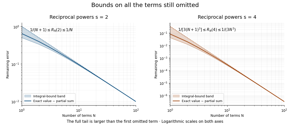
For a chosen absolute error target $\epsilon >0$, the sufficient condition is $N\ge ((s-1)\epsilon {)}^{-1/(s-1)}$, rounded upward to an integer. Thus $\epsilon =10^{-4}$ requires $N=10000$ by this bound for squares but only $N=15$ for fourth powers. This is a guarantee from an upper bound, not a claim that those are the smallest successful term counts.