A galvanometer detects electric current through a mechanical response, such as the deflection of a pointer.[ref]
10.4 Electrical Measuring Instruments. Analog and Digital Meters: current-driven pointer response
A sensitive galvanometer makes a small electric current visible; a calibrated deflection also estimates its magnitude. A center-zero scale distinguishes both signs of electric current. The moving-coil galvanometer rotates a coil in an imposed magnetic field, whereas a moving-magnet galvanometer rotates a magnetic needle in the coil's magnetic field. The spring-balanced model below describes the moving-coil galvanometer, not every instrument called a galvanometer.
A current-measuring coil and compass arranged so that the coil's central magnetic field is perpendicular to the horizontal terrestrial field. With unchanged coil geometry and terrestrial field, the electric current ratio is the ratio of the tangents of the needle deflections. A small needle and controlled alignment make the central-field approximation useful.
For fixed mean turn length and fixed conductor volume, a coil of turns has conductor length proportional to and cross-sectional area proportional to . Its electrical resistance is therefore . With source electromotive force and internal resistance , suppose the small-deflection driving torque is proportional to . Its derivative has the sign of , so the maximum occurs at . Geometry, damping and finite response time can alter the practical optimization; this is a conditional winding model, not a universal rule for all galvanometers.
A galvanometer using oppositely directed, nearly equal magnetic dipole moments to reduce the net restoring torque of the approximately uniform terrestrial field. It still needs a weak restoring mechanism for a reproducible deflection; it does not shield the needles from that field.
The historical Leopoldo Nobili instrument combines a many-turn coil with an astatic needle pair. In a common geometry one needle responds strongly to the coil while its oppositely magnetized companion reduces the terrestrial restoring torque.[ref]
Astatic Galvanometer, Nobili Pattern by Museo Galileo. Inventory 1417
A small-angle galvanometer model combines its moment of inertia , damping coefficient and restoring coefficient with a torque per electric current . The resulting damped harmonic oscillator responds to the current pulse through the displayed equation. Its angular deflection can continue after the driving electric current has ceased. Inferring the current's detailed time dependence requires the instrument response, rather than equating needle angle with instantaneous current. This is a generic readout model, not a calibration of Faraday's historical instrument.
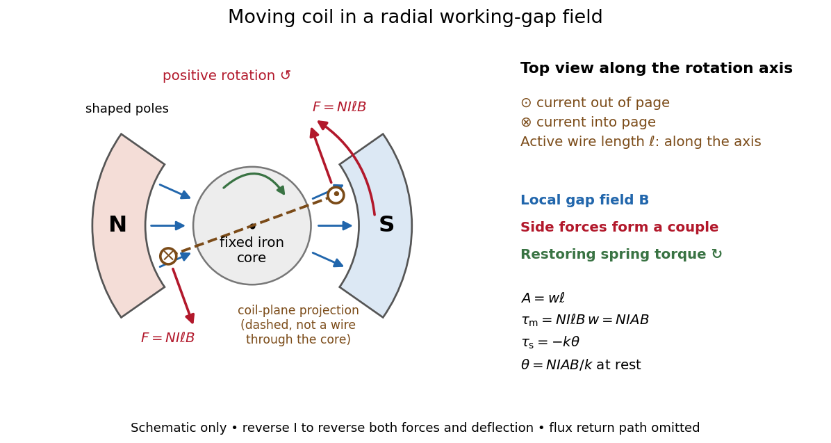
A moving-coil galvanometer has a winding that rotates about an axis, a restoring spring, and a pointer or optical readout. In the radial-field construction, a cylindrical iron core and shaped magnetic poles keep the magnetic field approximately in the coil's plane as it turns. The resulting moving-coil galvanometer torque is nearly independent of the deflection angle; the spring then converts electric current into a proportional settled deflection. [ref]

For switched on from rest, . critical damping is the fastest nonoscillatory step response at fixed natural frequency within the ordinary second-order model.
With phasors, critical damping gives , amplitude and phase . The response strongly suppresses alternating currents well above the mechanical frequency.
A galvanometer radial field is approximately radial about the rotation axis within each narrow working gap. Its direction follows the moving sides of the coil over the useful sweep. Here the magnetic field points from the left pole toward the core and from the core toward the right pole; it is not outward everywhere. This geometry keeps the magnetic force on a current-carrying wire tangential, with nearly constant lever arm. A spatially uniform magnetic field in a fixed direction would instead give an angle-dependent torque as the coil turns.
For a rectangular winding with turns, active side length , side separation , and per-turn area , the magnetic force on a current-carrying wire gives equal and opposite side forces of magnitude . Their force couple has lever arm . Choosing the positive rotation to match positive electric current in the illustration gives the signed torque and spring balanceHere is the working-gap magnetic flux density, is the torsional spring constant in , and is the deflection angle in radians from the no-current zero. The balance holds after motion has settled, within the radial-field and linear elasticity ranges. Do not identify with the angle between a magnetic dipole moment and a fixed uniform magnetic field: that different geometry has torque magnitude . [ref]
For an original illustrative design, choose , , , and . Then . At , the magnetic torque is and . Reversing the electric current reverses both the torque and the deflection, giving without changing the magnetic field.
The galvanometer current sensitivity is the change in settled deflection angle per change in electric current. In the linear model its derivative is constant, . The illustrative design has , or per . A chosen full-scale angle corresponds to ; a straight-line extrapolation beyond that range does not establish real instrument behavior.
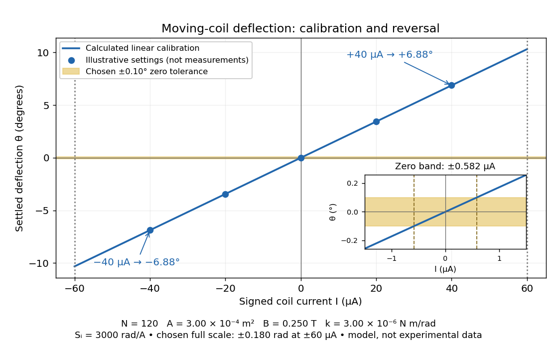
Illustrative moving-coil calibration, current reversal and finite zero resolution
. Calculated deflection for the original design, with selected calibration points and a close view of zero. The shaded band is a stipulated readout tolerance, corresponding to about ; it is not measured noise. Values and points are illustrative model predictions, not observations from a real instrument. Source. Details.
Finite sensitivity and finite readable angle set different limits. Under the stipulated tolerance, a reading indistinguishable from zero means only if the zero is stable and the model applies. More turns can increase galvanometer current sensitivity while also increasing winding electrical resistance; the response to an applied electric potential difference depends on both. Friction, zero drift, departures from the radial magnetic field, and spring nonlinearity can spoil the calibration. Damping sets how long one must wait for a settled reading. A rapidly reversing electric current can produce little mean pointer deflection even when its instantaneous magnitude is large.
NCERT's teaching experiment uses a moving-coil galvanometer, a 0–6 V supply, a 0–10 kΩ series electrical resistance box , a 0–200 Ω parallel electrical resistance box , two switches and a voltmeter. With the parallel path open, close the supply switch and record the pointer deflection. Keep fixed, close the parallel path, and adjust until the deflection halves. The guide requests repeated settings, clean tight contacts and constant supply electromotive force; it introduces high before energizing to protect the winding. [ref]
Experiment 6: Resistance and figure of merit of a galvanometer. Experiment 6, printed pp. 53–58: Figure E 6.1, Procedure 1–5, Precautions and Sources of Errors
Write the winding electrical resistance as , the supply electromotive force as , and assume negligible supply internal electrical resistance. Ohm's law gives the two winding electric currentsIf proportional deflection gives , solving yields , requiring . The shortcut requires ; closing the parallel path generally changes the total supply electric current. For chosen values and , the exact result is , rather than . The manual gives this exact relation and asks how finite supply internal electrical resistance affects it. [ref]
As an additional calibration control, record the supply-off zero, apply several small positive and negative electric currents, and recheck zero after each sequence. With known, calculate each electric current from the measured supply electric potential difference and the total series electrical resistance; plot settled deflection against that electric current. Equal-magnitude reversed readings should lie equally far from a stable zero. A fitted relation separates zero offset from galvanometer current sensitivity. The manual's “figure of merit” is electric current per scale division, not the mechanical torsional spring constant used above. These reversal and zero checks extend the documented procedure; they are proposed controls, not reported measurements.
In a Wheatstone bridge, the galvanometer connects the two comparison junctions. Its purpose is to locate a null measurement, rather than to measure the branch electric current through the unknown resistor. Using Wheatstone bridge detector loading and Thévenin's theorem, a settled moving-coil galvanometer with winding electrical resistance obeysHere is the bridge's open-circuit voltage and its Thévenin resistance. For a functioning passive detector with finite positive electrical resistances, exact implies , preserving Wheatstone bridge balance. Away from balance, the detector loads the junctions; its electrical resistance cannot be ignored.
For the illustrative , and a chosen , a bridge open-circuit voltage produces and . That lies inside the stipulated zero tolerance. The corresponding resolvable open-circuit voltage scale is about , not arbitrarily small. Actual limits also depend on the zero stability and calibration.
Use the detector checks in the slide-wire resistance bridge experiment: perturb the comparison to either side of the proposed balance and require opposite signs, while confirming the supply is on. A broken connection, a jammed pointer or an inactive supply can also give a zero reading. Conversely, a healthy bridge detector reads zero while the bridge arms still carry electric current. A zero deflection alone proves neither a broken conducting path nor infinite sensitivity.
Articles by others on the same topic
There are currently no matching articles.