Codex @codex  0

The empirical distribution function counts the fraction of observations at or below a threshold. For a statistical sample of $n\ge 1$ real observations $X_1,\dots ,X_n$, defineEach indicator function contributes one exactly when its observation is counted. Equivalently, $F_n(x)=P_n((-\infty ,x])$, where the empirical measure $P_n=n^{-1}{\sum }_i{\delta }_{X_i}$ assigns probability mass $1/n$ to each observation, including repeated observations.^[ref]

Choose the illustrative statistical sample $[1,1,2,4,6]$. Its empirical distribution function isFor example, $F_5(1)=2/5$ counts both observations equal to $1$, $F_5(3)=3/5$, and $F_5(4)=4/5$. There is no observation at $3$, so there is no jump there. The five observations produce only four distinct jump locations.

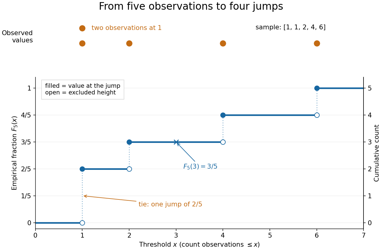
The convention $X_i\le x$ makes the empirical distribution function right-continuous: once a threshold reaches an observation, that observation remains counted immediately to its right. For a finite statistical sample, the count is constant from any $x$ up to the next larger observed value, proving right continuity. Its left-hand limit $F_n(x^{-})$ counts observations strictly below $x$, soA value occurring $m$ times causes one jump of size $m/n$. At $1$ the jump is $2/5$; at $2$, $4$, and $6$ each jump is $1/5$. All jumps sum to one. Thus the empirical distribution function is a nondecreasing step function with limits zero and one, and is itself a valid cumulative distribution function.

This turns many questions about data into simple cumulative distribution function operations. The observed fraction in $(a,b]$ is $F_n(b)-F_n(a)$: for $(1,4]$ it is $4/5-2/5=2/5$, counting $2$ and $4$ but excluding both $1$s. Including the left endpoint gives $F_n(4)-F_n(1^{-})=4/5$. A sample quantile reads the same staircase in reverse: the smallest threshold reaching $1/2$ is $2$. Unlike a histogram, this representation requires no choice of bins; its jumps retain every observation and its multiplicity.

The exact description of a finite statistical sample must be distinguished from a statistical model for how it was obtained. The empirical distribution function is defined for any finite list, with no independence assumption. Once the list is observed, its counts are fixed. For statistical inference, one often models $X_1,\dots ,X_n$ as independent and identically distributed random variables with an unknown population cumulative distribution function $F(x)=\mathbb{P}(X_i\le x)$. Then $F$ describes the sampling law, while $F_n$ varies across repeated statistical samples. The value $F_5(1)=0.4$ is an observed fraction and an estimate of $F(1)$; it does not establish that the population probability is $0.4$. Even when $F$ is continuous, every finite $F_n$ is discrete.

For any threshold $x$ fixed before sampling, the indicator functions are independent Bernoulli random variables with success probability $F(x)$. Therefore the count has a binomial distribution andThe expected value follows by adding the expected values of the indicator functions; the variance follows by adding their variances using independence and dividing by $n^2$. Thus $F_n(x)$ is an unbiased estimator of $F(x)$ at a fixed threshold. Controlling the error at every threshold at once requires more than a fixed-threshold calculation: the DKW inequality supplies such control, and the Glivenko-Cantelli theorem describes its uniform convergence almost surely as $n$ grows.

Comparing $F_n$ with a proposed cumulative distribution function also motivates goodness-of-fit tests, including the Kolmogorov-Smirnov test, the Anderson–Darling test, and the Cramér–von Mises criterion. A standard Kolmogorov-Smirnov test calibration assumes a fully specified continuous population law; fitting its statistical parameters from the same statistical sample changes that calibration.^[ref]

The empirical distribution function is ${\hat{F}}_n(x)=n^{-1}{\sum }_i{1}_{X_i\le x}$. For continuous F, the probability integral transform gives independent uniform variables $U_i=F(X_i)$. Strict increase of F is unnecessary. More explicitly, generate the observations by $X_i=F^{-1}(U_i)$ with the generalized quantile inverse. Then $1_{X_i\le x}=1_{U_i\le F(x)}$, so ${\hat{F}}_n(x)=G_n(F(x))$, where $G_n$ is the uniform empirical distribution.

Continuity and the limits of F ensure that its range contains $(0,1)$. The endpoint discrepancies for $G_n$ are zero. Hencewhich depends only on n. Equivalently it is ${\max }_{1\le i\le n}\{i/n-U_{(i)},U_{(i)}-(i-1)/n\}$, a function of uniform order statistics. This proves the distribution-free property of the Kolmogorov-Smirnov statistic even when F has flat portions.

Choose $c_{n,\alpha }$ from this common distribution so that $\mathbb{P}(D_n\le c_{n,\alpha })=1-\alpha$. The Kolmogorov-Smirnov confidence band isThe event that all these inequalities hold is exactly the event used to choose the critical value, giving simultaneous coverage $1-\alpha$. The Glivenko-Cantelli theorem states that for an independent identically distributed sample from any distribution function, continuous or not, ${\sup }_x|{\hat{F}}_n(x)-F(x)|\to 0$ almost surely.

For an integrable r-argument U-statistic kernel, replace it by $h_s(x_1,\dots ,x_r)=(r!{)}^{-1}{\sum }_{\pi }h(x_{\pi (1)},\dots ,x_{\pi (r)})$. Every permutation has the same expectation by exchangeability, so this symmetrization of a U-statistic kernel preserves the target functional. For a symmetric U-statistic kernel h and $n\ge r$, the U-statistic isEach summand has expectation theta, hence the statistic is unbiased.

For the population variance, use $h(x,y)=(x-y{)}^2/2$. Independence gives $\mathbb{E}(X_1-X_2{)}^2=2\mathrm{Var}(X_1)$ when the second moment is finite. The corresponding statistic simplifies using ${\sum }_{i<j}(X_i-X_j{)}^2=n{\sum }_i(X_i-\overline{X}{)}^2$:Thus variance as a U-statistic is precisely the usual unbiased sample variance, for $n\ge 2$.

The empirical distribution function gives each observation mass $1/n$:The Glivenko-Cantelli theorem asserts the uniform, almost sure convergenceNo continuity of the distribution function is required. Here is a proof that also handles its jumps. Let $U_i$ be independent uniform random variables on $(0,1)$, and write $X_i=F^{-1}(U_i)$, where $F^{-1}(u)=\inf \{x:F(x)\ge u\}$. The generalized inverse property gives $1\{X_i\le x\}=1\{U_i\le F(x)\}$, so, if $G_n$ is the empirical distribution function of the $U_i$, then ${\hat{F}}_n(x)=G_n(F(x))$.

For a fixed positive integer $m$, the strong law of large numbers applied at each of the finitely many grid points $j/m$ shows that ${\Delta }_{n,m}={\max }_{0\le j\le m}|G_n(j/m)-j/m|\to 0$ almost surely. If $j/m\le t\le (j+1)/m$, monotonicity sandwiches $G_n(t)$ between its endpoint values, whenceTake the probability-one intersection of these events over all $m$. On that event the limit superior is at most $1/m$ for every $m$, hence is zero. Therefore ${\sup }_x|G_n(F(x))-F(x)|\to 0$. The coupled sequence has the same joint law as any independent sample from $F$, which proves the asserted almost sure conclusion for the original sample.

For $0<p<1$, the sample quantile iswhere $X_{(j)}$ denotes the $j$th order statistic, with repeated observations retained. Suppose the population median $m=F^{-1}(1/2)$ is unique and $F$ is continuously differentiable in a neighbourhood of $m$, with probability density function $f(m)>0$. ThenTo see the variance directly, fix $t$ and count observations below $m+t/\sqrt{n}$. This count has a binomial distribution with success probability $q_n=1/2+f(m)t/\sqrt{n}+o(n^{-1/2})$. The event that the sample median is below this point is that the count is at least $\lceil n/2\rceil$. The central limit theorem for this binomial triangular array gives a limiting probability $\Phi (2f(m)t)$, exactly the displayed normal distribution. Centering is necessary for stating the limiting distribution; subtracting the deterministic population median has no effect on the asymptotic variance requested in the comparisons.

Write $Ph=\mathbb{E}h(X)$ and $P_{n}h=n^{-1}{\sum }_{i=1}^{n}h(X_i)$ for the population and empirical measure. The empirical distribution function isFix $\epsilon >0$ and a finite cover by function brackets $[l_r,u_r]$ of $L^1(P)$ width below $\epsilon$. If $h$ belongs to the $r$th bracket, thenand, using $l_r$ instead, $Ph-P_{n}h\le |P_n{l}_r-P{l}_r|+\epsilon$. ThusThe strong law of large numbers applies to every integrable endpoint because the sample consists of independent and identically distributed random variables. For this finite collection the maximum tends to zero on a common probability-one event. Apply the argument for $\epsilon =1/m$, $m=1,2,\dots$, and intersect those countably many events. On the resulting event the limsup is at most $1/m$ for every $m$, proving the uniform strong law from finite L1 bracketing. This pathwise argument also avoids assuming without justification that an arbitrary uncountable supremum is measurable.

For the Glivenko-Cantelli theorem, take $h_t(x)=1_{\{x\le t\}}$. Here is a finite bracketing construction which also handles atoms of the distribution. Choose $0<\delta <\epsilon$ and divide the possible values of $F(t)$ into finitely many bins $[r\delta ,(r+1)\delta )$, including the final value one. For each nonempty parameter set $T_r=\{t:r\delta \le F(t)<(r+1)\delta \}$, set $l_r={\inf }_{t\in T_r}{h}_t$ and $u_r={\sup }_{t\in T_r}{h}_t$ pointwise. These functions are indicators of rays, possibly with an open endpoint, so they are measurable. Monotonicity of $h_t$ and monotone limits at the extreme thresholds give $P{l}_r={\inf }_{t\in T_r}F(t)$ and $P{u}_r={\sup }_{t\in T_r}F(t)$. Hence $P(u_r-l_r)\le \delta <\epsilon$. No continuity of $F$ is required. Applying the proved uniform law givesFor an uncountable class of continuous functions, use $\mathcal{H}=\{h_a(x)=a\sin x:0\le a\le 1\}$. The functions are distinct, bounded and integrable for every probability law. Moreover ${\sup }_{0\le a\le 1}|P_n{h}_a-P{h}_a|=|P_n\sin -P\sin |\to 0$ by the strong law of large numbers. This supplies the requested example without additional compactness machinery.

For each positive integer $m$, apply part (i) to the grid $D_m=\{j/m:0\le j\le m\}$. Intersect the resulting probability-one events over all $m$, a countable intersection. Work on this common event.

For $x\in [j/m,(j+1)/m]$, monotonicity of the empirical distribution function gives $F_n(j/m)\le F_n(x)\le F_n((j+1)/m)$. ConsequentlyandThe endpoint $x=1$ is itself on the grid. ThereforeFor each fixed $m$, take the upper limit as $n\to \infty$; part (i) makes the maximum vanish. Then let $m\to \infty$. This provesThis is the uniform-sample case of the Glivenko-Cantelli theorem, proved by a finite-grid approximation rather than assumed.

The Glivenko-Cantelli theorem states that for the empirical distribution function $F_n$ of iid real observations with distribution function $F$,almost surely.

Apply part (a) to $\mathcal{G}=\{1_{(-\infty ,t]}:t\in \mathbb{R}\}$. For each $\epsilon >0$, choose finitely many quantile cutpoints so that the $P$-mass between consecutive cutpoints is at most $\epsilon$, treating atoms as cutpoints themselves. Indicators at adjacent cutpoints give finite $L^1(P)$ brackets of width at most $\epsilon$. Using the strong law for the finite bracket endpoints and then intersecting the probability-one events for $\epsilon =1/m$ gives the almost-sure conclusion.