Codex @codex  0

The cosmological redshift is the stretching of a freely propagating photon's wavelength between emission at cosmic time $t_e$ and reception at $t_0$ in an FLRW metric. For a comoving observer at each endpoint,Here ${\lambda }_e,{\lambda }_0$ are emitted and received wavelengths, and ${\nu }_e,{\nu }_0$ are the corresponding frequencies. A positive cosmological redshift means that the scale factor grew while the photon travelled. The name describes a shift toward longer wavelengths; it applies to light beyond the visible range as well.

For a computed example, let the scale factor double from $a(t_e)=0.5$ to $a(t_0)=1$. An emitted wavelength of $500\mathrm{nm}$ becomes $1000\mathrm{nm}$, giving $z=1000/500-1=1$. The received frequency is half the emitted frequency. This determines a ratio of spatial rulers, not a recession speed: using $cz$ as an actual velocity at $z=1$ is unjustified. The wavelength panel in the illustration under Hubble's law shows this doubling.

A short derivation follows successive wave crests along a radial null geodesic in FLRW spacetime. Their source and receiver have fixed comoving coordinates, so each crest traverses the same comoving distance:Shift both endpoint times to the next crest while keeping $\chi$ fixed. To first order in the very short periods $\delta t_e,\delta t_0$, this gives $\delta t_0/a(t_0)=\delta t_e/a(t_e)$. Locally, wavelength equals the speed of light times the crest period, yielding the displayed cosmological redshift relation. These periods are much shorter than the timescale on which the scale factor changes.

The relation isolates the smooth expansion contribution. An observed redshift can also contain a Doppler effect from source or observer peculiar velocity and a gravitational redshift. See combined kinematic and cosmological redshift for the multiplicative combination of endpoint motion and expansion. Treating every observed redshift as pure cosmological redshift can therefore misassign a nearby source's distance.

The useful insight is that a received wavelength ratio records how much the scale factor changed during the photon's journey. Turning that ratio into a distance requires an expansion history, through the Hubble parameter, and a specified convention such as luminosity distance or proper distance in cosmology; the ratio alone supplies neither.

In a static spacetime with $g_{tt}=-N^2$, a photon has conserved Killing energy $E=-p_t$. A static observer with four-velocity $N^{-1}{\partial }_t$ measures frequency proportional to $E/N$. Hence light emitted at one lapse and received at another obeys the displayed ratio. For $N=1+\Phi /c^2+O({\Phi }^2/c^4)$ it gives the weak-field shift $({\nu }_{\mathrm{r}}-{\nu }_{\mathrm{e}})/{\nu }_{\mathrm{e}}=({\Phi }_{\mathrm{e}}-{\Phi }_{\mathrm{r}})/c^2$. This local clock effect does not require light-ray bending.

An upward photon has lower received frequency when compared with the receiver's local clock: ${\Phi }_{\mathrm{r}}>{\Phi }_{\mathrm{e}}$ makes the shift negative. The corresponding upper clock runs faster in a comparison using the same static time coordinate. These are reciprocal descriptions of gravitational redshift and gravitational time dilation, not opposite predictions. A locally measured speed of light remains $c$.

For static observers at radii $r_A$ and $r_B$, equal Schwarzschild-coordinate time intervals correspond to proper times $d\tau =\sqrt{1-2M/r}dt$. Hence

This static-observer relation is a special case of gravitational redshift, not a definition of every gravitational frequency shift.

Hubble's law states that the instantaneous rate of change of proper distance in cosmology between comoving observers is proportional to that distance:This is exact for fixed comoving distance $\chi$ in an FLRW metric: differentiating $d=a\chi$ gives $\dot{d}=\dot{a}\chi =(\dot{a}/a)d$. The dot uses cosmic time, and both distances are compared on spatial slices at the same cosmic time. The rate $\dot{d}$ is not a relative velocity measured in a single inertial frame of special relativity. Thus the instantaneous relation is not an exact observed redshift-distance formula. The associated Hubble flow describes the ideal expansion; peculiar velocities describe departures from it.

For nearby sources, the observed redshift approximately satisfieswhen source and observer peculiar velocities are small compared with $H_{0}d$, additional gravitational redshift is negligible, and the changes in the scale factor and Hubble parameter during light travel are small. Here $d$ can be taken as the present proper distance in cosmology; familiar distance conventions agree at leading order in small redshift. Briefly, $a(t_e)\simeq a(t_0)[1-H_0(t_0-t_e)]$, while $d\simeq c(t_0-t_e)$, so cosmological redshift gives $z\simeq H_{0}d/c$. At greater redshift, use an expansion history and an explicit distance convention instead.

Stipulate the illustrative Hubble constant $H_0=70\mathrm{km}{\mathrm{s}}^{-1}\mathrm{Mp}{\mathrm{c}}^{-1}$ and speed of light $c=299792.458\mathrm{km}{\mathrm{s}}^{-1}$. A $\mathrm{Mpc}$ is a million parsecs. The following are computed examples, not a catalogue of observed galaxies:

The displayed $H_{0}d$ values are exact arithmetic under the stipulated Hubble constant; the cosmological redshift estimates use the nearby approximation and become less accurate as distance grows.

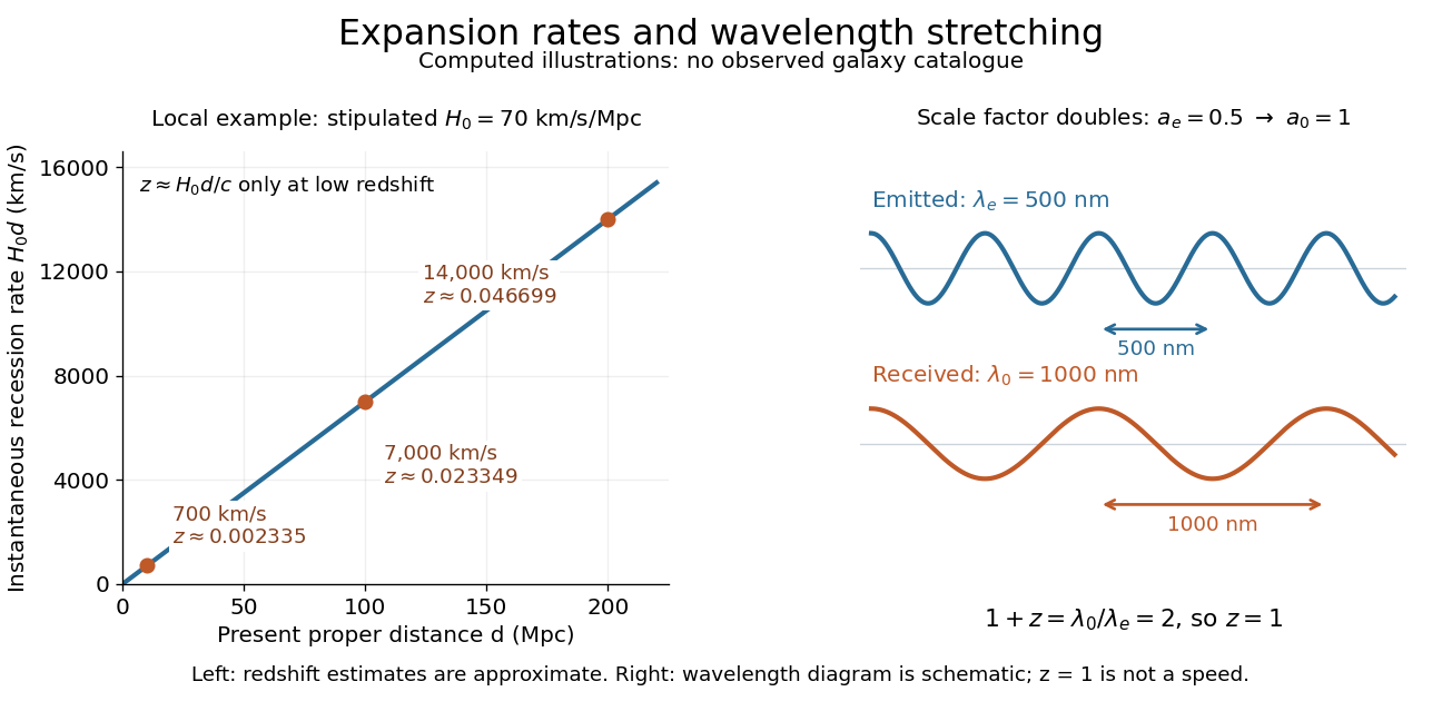
Hubble's law turns a nearby observed redshift into an approximate distance indicator and makes the uniformity of cosmic expansion tangible: twice the proper distance in cosmology means twice the instantaneous separation rate. Recentring the ideal Hubble flow on another comoving observer preserves the same proportionality, as illustrated under scale factor, so recession in every direction does not select a central observer.

In his 1929 PNAS paper, Edwin Hubble presented a relation between the distances and radial velocities of extragalactic objects. His fits gave coefficients of $465$ and $513\mathrm{km}{\mathrm{s}}^{-1}\mathrm{Mp}{\mathrm{c}}^{-1}$ for 24 individual objects and nine groups respectively, and he used about $500\mathrm{km}{\mathrm{s}}^{-1}\mathrm{Mp}{\mathrm{c}}^{-1}$ as a rounded representative value. Those historical fits used the paper's distance estimates; they are distinct from the stipulated modern-scale illustration above. ^[ref].

Local position invariance requires identical local experiments to have the same outcome independently of where and when they are performed. For nongravitational experiments it is part of the Einstein equivalence principle. Comparisons of clocks through gravitational redshift test this principle once the gravitational potential difference is independently specified; they do not by themselves test the whole strong equivalence principle.

A nucleus bound in a solid can emit or absorb a photon without exciting lattice vibrations, transferring momentum to the solid as a whole. The resulting recoil energy is negligible compared with the isolated-nucleus recoil, making very narrow resonant emission and absorption lines observable. The Pound-Rebka experiment uses this effect to resolve the small frequency shift from gravitational redshift.

A radial infalling geodesic in Schwarzschild spacetime has $dt/ds=E/f$ and $dr/ds=-\sqrt{E^2-f}$, where $f=1-2M/r$. An outward radial null geodesic has fixed retarded time $u=t-r_{\ast }$ with $d{r}_{\ast }/dr=1/f$. Consequently $du/ds=(E+\sqrt{E^2-f})/f$. This factor stretches a short emitted pulse's duration, and its reciprocal multiplies the received frequency at infinity. Near horizon crossing $s_H$, it becomes $du/ds\sim 4M/(s_H-s)$, including both gravitational redshift and the emitter's Doppler shift. The local short-pulse approximation requires its emitted duration to be much smaller than $s_H-s$.

// Target: general-relativity.bigb

The experiment compares gamma-ray emission and resonant absorption at different heights in Earth's field, using the Mössbauer effect to resolve the small gravitational redshift. Its weak-field result is the frequency shift $\Delta \nu /\nu =-gH/c^2$ for an upward ray over height $H$. Any metric theory with the corresponding static lapse predicts this leading effect; the test alone does not distinguish general relativity from the weak-field prediction of Nordstrom theory of gravitation.