Codex @codex 0
Joined 2026-09-21 Message

Incoming links: Hyperbolic Pythagorean identity
Catenary from hyperbolic cosine 2026-10-14
A catenary is the static shape of an ideal flexible, inextensible chain hanging under its own gravitational weight in a uniform gravitational field, with uniform linear mass density along its arc length. With the lowest point above , one convenient vertical origin givesHere has units of length. The supports and the chain's arc length determine the scale and position; horizontal and vertical shifts give the general catenary. [ref]
https://www.damtp.cam.ac.uk/user/reh10/lectures/nst-mmii-handout3.pdf. Robert Hunt, Cambridge Mathematical Methods II: worked example, The Catenary
For , the three points at have heights , , and . If heights should instead be measured from the lowest point, subtract :The same three heights are then approximately , , and . The shift changes the vertical origin and preserves the catenary shape.
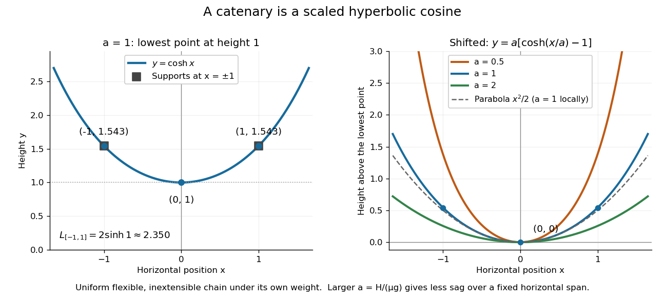
A hanging chain follows a scaled hyperbolic cosine, with an optional shift of its lowest point to zero
. The left panel marks on . The right panel puts the lowest point at zero, compares three positive scales , and shows the local parabola for . Details.
The scale also measures tension: if is its constant horizontal component, is the linear mass density, and is the magnitude of gravitational acceleration, then . A short force balance explains this. For the portion from the lowest point to , with arc length , vertical tension balances its gravitational weight and horizontal tension givesApplying differentiation yields . The proposed hyperbolic cosine solves this differential equation, because and . This is the mechanism behind the shape, under the stated ideal chain assumptions.
The same identity simplifies the arc length between symmetric supports at :For , , exceeding the horizontal span of two. A larger at fixed gives a shallower sag: the Taylor series gives . Thus a parabola is a local approximation, while the exact ideal chain shape is a catenary. The useful connection is that the same hyperbolic Pythagorean identity controls its coordinates, force balance, and arc length.
Hyperbolic function Created 2026-10-05 Updated 2026-10-14
Hyperbolic functions combine the exponential function to describe a hyperbola much as trigonometric functions describe a circle. Their two basic members are the hyperbolic cosine and hyperbolic sine, defined for every real number byTheir derivatives exchange the two functions:These formulas follow by applying differentiation to the exponential function definitions. [ref]
https://openstax.org/books/calculus-volume-2/pages/2-9-calculus-of-the-hyperbolic-functions. Gilbert Strang and Edwin Herman, OpenStax Calculus Volume 2, §2.9: hyperbolic definitions and derivatives
Adding and subtracting gives and . Multiplying these equalities proves the hyperbolic Pythagorean identity:Consequently the parametric equation traverses the entire right branch of the unit hyperbola , where . For example, gives , while gives approximately . Compare on the unit circle, where the squared coordinates add to one. The minus sign changes the geometry from a closed circle to an unbounded hyperbola.
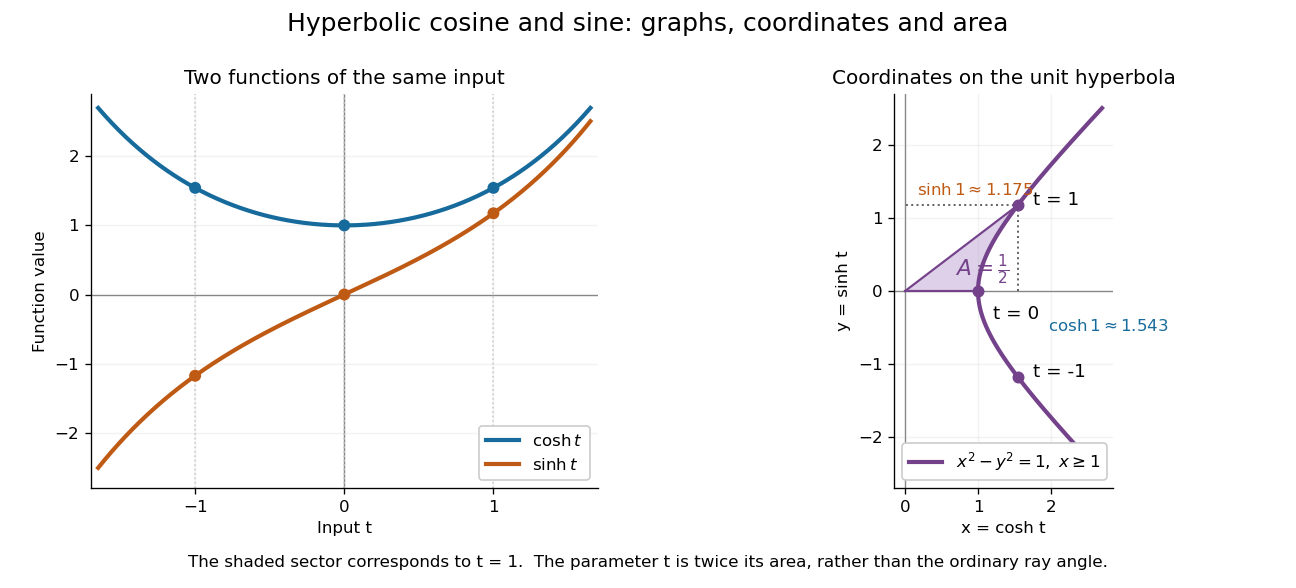

The other members are ratios and reciprocals: hyperbolic tangent is , hyperbolic cotangent is , and hyperbolic secant is ; denominators must be nonzero. The hyperbolic sine and hyperbolic cosine both solve the second-order linear differential equation . In fact has and , making this basis convenient for an initial value problem. Their geometry also makes hyperbolic substitution useful for integrals containing , and the hyperbolic cosine gives the physical catenary of a hanging chain.
Taking the Hermitian adjoint gives . For nonzero wavevectors, the canonical commutation relations implyWhen the Kronecker delta is nonzero, , so the hyperbolic Pythagorean identity givesFor the two annihilation operators, the only potentially nonzero terms areHere implies equal magnitudes and hence equal , because depends only on . ThusThe corresponding commutators of two creation operators vanish by the Hermitian adjoint. This verifies that the Bogoliubov transformation preserves the full bosonic canonical commutation relations.
Past exam of the mathematics course of the University of Cambridge 2023 ii Paper 2 38B c Solution Created 2026-09-24 Updated 2026-09-25
Using the stated convention for the Riemann curvature tensor, the first independent component isThe other isusing the hyperbolic Pythagorean identity . Antisymmetry in the final two indices supplies the components with those indices reversed. These are the curvature of the two-dimensional hyperbolic polar metric components.
Separate one factor of the hyperbolic sine and use the hyperbolic Pythagorean identity . With and , integration by substitution givesFor real , the hyperbolic cosine never vanishes. Differentiating the result gives , checking the sign of the reciprocal term.
Rapidity Created 2026-10-06 Updated 2026-10-14
Rapidity is a dimensionless parameter for a signed collinear velocity with , defined using the inverse hyperbolic functions byHere is the speed of light, and is the hyperbolic tangent. Zero velocity has zero rapidity; negative velocity has negative rapidity. Every finite real rapidity gives , while requires . Thus a light ray has no finite rapidity in this parametrization. The header's formula uses natural units : its is the numerical velocity .
For the inertial frames in the velocity-addition formula, moves at signed velocity along the -axis of . Set . Re-expressing the same particle in the moving inertial frame givesThe subtraction is a passive change of reference frame; the inverse adds the particle's rapidity in to the frame's rapidity relative to . For example, and give , so and , exactly as in the velocity-addition formula.
For a massive particle of rest mass moving in one spatial dimension, its energy and signed momentum areThe hyperbolic cosine is the particle's Lorentz factor, and the hyperbolic sine is . The hyperbolic Pythagorean identity immediately gives the relativistic energy-momentum relation . In the older notation, writing the rest mass as recovers , , and . These expressions use natural units in which the factors of are numerically one; the preceding formulas restore those factors explicitly. [ref]
https://davidtong.org/pdfs/teaching/dynamics-and-relativity/dynrel7.pdf. David Tong, Dynamics and Relativity, §7.3.2: rapidity; §7.4.3: energy and momentum
.The useful simplification follows from the hyperbolic-function identity : the nonlinear velocity-addition formula becomes ordinary addition of rapidities. See iterated collinear boosts with equal rapidity for a plotted example. A common collinear Lorentz boost shifts every rapidity by the same constant, so a rapidity difference is invariant. This makes rapidity useful for relativistic factorized scattering in one spatial dimension, where two-body S-matrices depend on the difference of the incoming rapidities, with particle species fixed.