An optical lens is a transparent element, or assembly of elements, that redirects a bundle of light rays to form images or change how the bundle spreads. In an ordinary glass optical lens, refraction at the surfaces provides the redirection: their changing normal vectors make Snell's law bend different light rays by different amounts. A converging optical lens brings incoming light rays parallel to its optical axis toward an optical focus; a diverging optical lens makes them spread as if from an optical focus on the incoming side. [ref]
https://openstax.org/books/university-physics-volume-3/pages/2-4-thin-lenses. Ling, Sanny and Moebs, OpenStax University Physics Volume 3, §2.4: Thin lenses
.For a usual glass thin lens in air, a form thicker at the centre than at the edges normally converges, with positive focal length; one thinner at the centre normally diverges. Shape alone is insufficient: the refractive index relative to the surroundings also matters, as the lensmaker's equation shows. An aperture selects which light rays pass; an optical lens also changes their directions. The distinction explains how an optical camera can gather light from one object point over many incoming directions and deliver it to one image location.
The beautiful simplification is that an entire bundle can be characterized by a focal length, and two constructed light rays can locate an image. The thin lens examples below turn that geometry into a prediction of image position, orientation and transverse magnification. A real optical lens retains optical aberrations and diffraction, so the construction is a useful leading model rather than an exact solution of Maxwell's equations.[ref]
Early mathematical treatments include Johannes Kepler's 1611 Dioptrice, whose title explicitly concerns vision through newly invented instruments using transparent glass, and René Descartes's 1637 La Dioptrique, whose seventh discourse discusses improving vision with shaped glass. These are landmarks in explaining and designing optical instruments, rather than dates for the invention of the optical lens. [ref]
https://www.e-rara.ch/zut/content/titleinfo/120202. Kepler, Dioptrice, 1611, original edition digitized by ETH-Bibliothek
; [ref]https://classiques.uqam.ca/classiques/Descartes/dioptrique/dioptrique.html. Descartes, La Dioptrique, 1637, seventh discourse, UQAM text edition
.An optical focus is a point where a specified bundle of light rays converges, or where its backward extensions meet. For a converging thin lens receiving light rays parallel to the optical axis, the rear optical focus is when the thin lens is at ; its front optical focus is . An object's image is generally elsewhere: the optical focus describes the parallel incoming bundle, while the thin lens equation locates the image for a finite object distance.
The focal length specifies the signed distance from an ideal thin lens to its optical focus for incident light rays parallel to the optical axis. A converging thin lens has , with a rear optical focus beyond the thin lens; a diverging thin lens has , with a virtual optical focus on the incoming side. The focal length is a property of the optical lens in its specified surroundings, not the image distance for every object. For example, a converging thin lens with images an object away at , as computed below. [ref]
https://www.feynmanlectures.caltech.edu/I_27.html. Feynman, Leighton and Sands, The Feynman Lectures on Physics I, §§27-3–27-4
.The optical power is reciprocal signed focal length, . With expressed in metres, optical power is expressed in dioptres: gives , while gives . The sign distinguishes converging and diverging optical lens elements; the magnitude measures how strongly they change the direction of a light ray at a given height. [ref]
https://openstax.org/books/college-physics-2e/pages/25-6-image-formation-by-lenses. Urone and Hinrichs, OpenStax College Physics 2e, §25.6: Optical power and diopters
.For two ideal thin lens elements in contact in air, optical powers add: . Thus and combine to give , or . Separation changes the rule: for two ideal thin lens elements separated by in air, their equivalent optical power is . The contact rule is the case.[ref]
Lecture Notes on Geometrical Optics. §J: Composite lenses
A dioptre, also spelled diopter, is the unit of optical power equal to one reciprocal metre. In , convert focal length to metres before taking the reciprocal: gives , not . A dioptre measures focusing strength, distinct from the transverse magnification of an image.
A thick lens retains the separation of its refracting surfaces when predicting image formation. In the paraxial approximation with air on both sides, object and image distances measured from the respective principal planes satisfy the familiar imaging equation. Measuring instead from one mechanical centre generally introduces an error.[ref]
Refracting systems (details), University of Tennessee physics teaching resource. University of Tennessee physics teaching resource, Refracting systems (details), final paragraph: object and image distances must refer to the principal planes
The two principal planes are reference planes that represent a centred imaging system in the paraxial approximation. In air on both sides, measure object distance from the front principal plane, image distance from the rear principal plane, and focal length from each principal plane to its corresponding optical focus. They need not coincide with a surface or mechanical centre. Their signed separation matters in the Bessel lens displacement method.[ref]
Refracting systems (details), University of Tennessee physics teaching resource. Refracting systems (details), definition of principal planes, unit lateral magnification, and final imaging equation
A thin lens models an optical lens by collapsing its refracting surfaces into one plane, neglecting thickness relative to the relevant radius of curvature values and object and image distances. Here use an ideal converging thin lens in air and the paraxial approximation: light rays make small angles with the optical axis, so Snell's law can be linearized using the small-angle approximation. Equal surrounding refractive indices on both sides give the familiar symmetric equation.[ref]
Put the thin lens at , with incident light travelling to the right. An object at has . The image coordinate is : for a real image and for a virtual image. The converging thin lens has focal length , and heights are signed relative to the optical axis. The thin lens equation and transverse magnification areThe expression for requires . Negative transverse magnification means inverted; positive transverse magnification means upright. Remember that the positive distance differs in sign from the object's coordinate . [ref]
https://openstax.org/books/university-physics-volume-3/pages/2-4-thin-lenses. Ling, Sanny and Moebs, OpenStax University Physics Volume 3, §2.4: Sign conventions
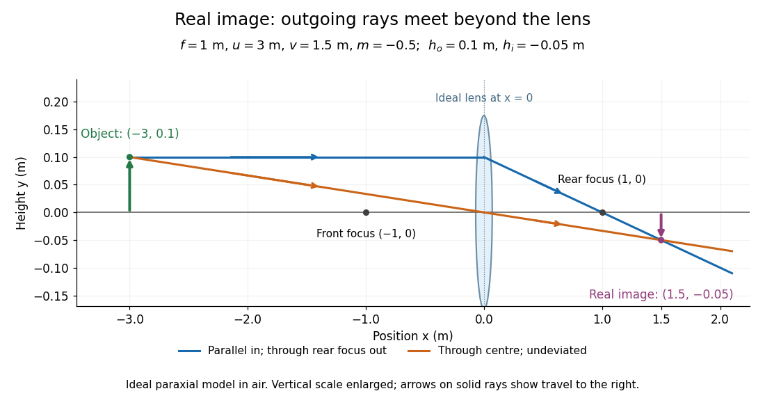
.For focal length , object distance , and object height , calculation givesThe real image is inverted, half as tall, and located to the right of the thin lens. A screen at that position receives the image because the outgoing light rays actually meet there.

For the same focal length and object height , move the object inside the front optical focus, to . ThenThe virtual image is upright, twice as tall, and apparently to the left of the thin lens. Outgoing light rays still travel to the right; only their backward extensions intersect at the virtual image. A screen there cannot collect that image from the outgoing bundle. This geometry explains why a converging optical lens can act as a magnifier when held close to an object. [ref]
https://openstax.org/books/college-physics-2e/pages/25-6-image-formation-by-lenses. Urone and Hinrichs, OpenStax College Physics 2e, §25.6: Virtual images inside the focus
.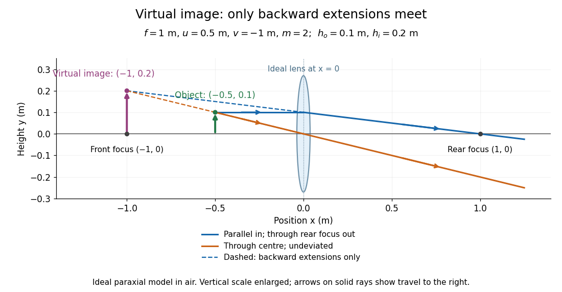

Both diagrams use two rules for ray tracing. A light ray from the object's tip parallel to the optical axis reaches the thin lens at and exits along the straight line through the rear optical focus . Another light ray through the centre continues undeviated in the ideal thin lens model. Their intersection, or the intersection of their backward extensions, locates the image tip. [ref]
https://openstax.org/books/university-physics-volume-3/pages/2-4-thin-lenses. Ling, Sanny and Moebs, OpenStax University Physics Volume 3, §2.4: Ray tracing
.A short geometric proof outline makes the signs transparent. The two outgoing straight lines areFor nonzero , equating their heights at gives , hence the thin lens equation; the centre light ray gives , hence the transverse magnification. This derives the image equations from the ideal ray tracing rules, whose physical justification comes from Snell's law in the paraxial approximation.
At , the two outgoing straight lines are parallel: there is no finite image position. For the real image has ; for the virtual image has . These cases let an optical camera designer choose a receiving position and let a user understand a magnifier. An actual optical lens has finite apertures, which cause diffraction and impose diffraction-limited resolution; optical aberrations can further blur the image. The diagrams are ideal geometrical optics, with exact coordinates within that model, rather than exact predictions of Maxwell's equations. [ref].
Use positive distances for a real incident object and a real outgoing image. The first thin lens makes an image at . The second has object distance , possibly negative, and the thin lens equation gives the displayed expression. At it becomes with . For , a real final image requires both and ; the inequality alone is insufficient when .
For two thin converging lenses, the first lens may form its would-be image beyond the second lens. The rays entering lens 2 then converge, so its Cartesian real-object distance is negative. Apply separately at each lens rather than treating that intermediate focus as an object upstream. In the example with separation , and . Multiplying the two signed transverse magnifications determines final inversion; a positive outgoing image distance means a real image.
For an optical element, a virtual object is a point toward which incident rays already converge, so they would meet beyond the element if it were removed. It is distinct from a virtual image, which is an apparent origin of outgoing rays. In the real-is-positive thin-lens convention, a virtual object beyond the lens has , and . Thus gives a real image in the rear focal plane of a converging lens.
For a converging thin lens forming a real image of a real object, let be positive distances from the lens and the focal length. Set and , measuring from the neighboring focal points. Substituting into gives , so . Other object-image geometries require an explicitly consistent signed-distance convention.
The Bessel lens displacement method measures a converging thin lens's focal length by moving only the optical lens between a fixed object and screen. If their separation is , two settings give sharp real images: one enlarged, the other reduced. Read their separation on an optical bench, then calculateThe two settings exchange object and image distances, so their signed transverse magnifications are reciprocals. This makes the experiment a visible test of conjugate optical planes as well as a focal length measurement.[ref]
For an original stipulated example, put the object at , the screen at , and take an ideal thin lens with . Its two settings are and , with . The transverse magnifications are and : both real images are inverted. An object tall would give signed image heights and . Conversely, stipulated readings and give . These are model calculations, not measured data or a manufacturer's calibration.
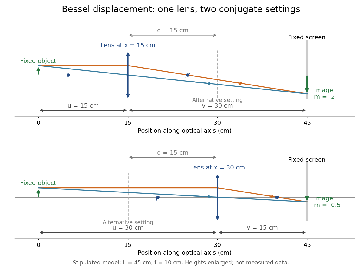

A fixed offset between a carrier's reference mark and an ideal thin lens plane cancels when subtracting the two carrier readings. That useful cancellation does not make a thick lens equivalent to one unknown optical centre: its two principal planes can be separated. The Bessel lens displacement experiment below makes this limitation explicit.
Place a converging thin lens at coordinate between the object at and the screen at . In air and the paraxial approximation, the required object and image distances are and . The thin lens equation gives a quadratic equation:Its discriminant is . For , the two roots and their separation areBoth roots lie inside , and both object and image distances exceed . The two roots therefore describe finite real images on the screen. Exchanging the roots exchanges ; from transverse magnification ,The image-height ratio between the enlarged and reduced settings is , rather than .
At , the roots coincide: , , and . There is one setting, not two separately measurable settings. For the discriminant is negative, so no position between the fixed object and screen gives a sharp real image there. This does not forbid a real image elsewhere if the screen is moved. Another short proof observes that has maximum at ; the focusing requirement is possible exactly when .
KIT's teaching apparatus uses a glass spoke-wheel or test negative as the object, a halogen lamp with an illuminating optical lens, an imaging optical lens, a screen and a triangular rail with a position scale. The illuminating optical lens concentrates the lamp filament's image on the imaging optical lens's centre; translucent paper checks that illumination. This reduces the contribution of peripheral light rays and their spherical aberration. The instructions require fixed object-screen separation exceeding , at least ten displacement measurements, and separate red- and blue-filter measurements to test chromatic aberration.[ref]
Brennweite dünner Linsen by Karlsruhe Institute of Technology, Faculty of Physics teaching laboratory. Karlsruhe Institute of Technology, Brennweite dünner Linsen, Durchführung and Aufgaben 1a and 2: target, illumination check, rail readout, repeated Bessel measurements and colour controls
The following measurement protocol elaborates that apparatus rather than reporting additional KIT results. Align the target centre, optical lens and screen normal along one optical axis; measure between the target pattern plane and receiving screen face. Lock the target and screen. Slide the imaging optical lens to obtain the enlarged real image, then the reduced real image, reading the same carrier reference mark at each setting. Record and for each pair. Record corresponding target and image intervals to test the reciprocal transverse magnifications independently; merely observing different image sizes is a weaker test.
Use the same central target detail to judge best optical focus. Bracket each setting by moving through both visibly blurred sides, repeat from both travel directions, and record the accepted position range as well as repeat scatter. Rail divisions set a readout limit but do not alone specify focusing uncertainty. Check scale calibration, carrier play and drift; a common additive carrier offset cancels in , whereas scale-factor error remains. Keep illumination, aperture, target, screen and optical lens orientation fixed within a series. Change the aperture and colour filter in separate control series: spherical aberration and chromatic aberration can shift the apparent best optical focus, while a very small aperture introduces stronger diffraction and makes focus discrimination harder. Record these settings alongside the inferred focal length, rather than interpreting all disagreement as random measurement error.
For a rigid thick lens in air, let be the signed separation of its rear and front principal planes along the direction of propagation. Then the positive object and image distances measured from the principal planes obey . Translating the whole assembly without reversing it moves both principal planes equally, so the measured carrier displacement still equals the difference of the two solutions for . The same algebra therefore givesHere is the effective focal length measured from the principal planes. This deduction uses the principal-plane imaging equation, not the uncorrected thin lens formula.[ref]
Refracting systems (details), University of Tennessee physics teaching resource. Refracting systems (details), principal-plane definition and final paragraph on object/image distances
Mechanical centre thickness is not generally . Record thickness and optical lens orientation, but use a justified bound or model for if it matters at the claimed precision. The two readings alone cannot determine both and unknown ; cancelling a carrier offset does not cancel this limitation.For small measurement errors, write . Its partial derivatives and first-order propagation of uncertainty areHere the values are standard deviations used to describe uncertainty, and is the covariance. Independent carrier-reading errors give ; correlated readings require the term . Averaging repeated independent pairs reduces the random component of the uncertainty of the mean, but does not remove calibration or model errors.
As a stipulated uncertainty calculation, let , , and , with all three input errors independent. Then , , and . The result would be with this standard uncertainty in the stipulated thin lens model; these numbers are not a measured uncertainty budget. A small neglected principal-plane separation gives an additional first-order bias , distinct from that random budget.
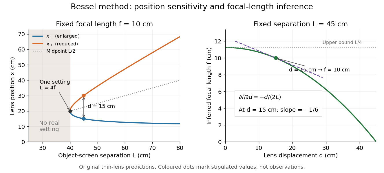
Bessel lens displacement method: merging settings and focal length sensitivity
. Original ideal-model curves. Left: settings versus object-screen separation for fixed ; below there is no real setting on the fixed screen. Right: inferred focal length versus measured displacement at fixed , with its tangent at the stipulated . The curves are predictions, not experimental points. Details.
The two kinds of sensitivity must be distinguished. At fixed focal length,These derivatives diverge as approaches from above: a small change in object-screen spacing strongly changes the separation of the two settings. Yet the inferred focal length's displacement sensitivity tends to zero. That does not make coalescing settings easy to measure. For fixed , define the axial mismatch between the predicted real image and the screen as , for . At a focused setting,Near , moving the optical lens changes this mismatch only weakly, making visual discrimination of the two settings difficult. At the example's settings and , so equal carrier motion produces different axial defocus responses. This is an axial mismatch calculation, not a full prediction of perceived image sharpness.
Choose sufficiently above to separate the two accepted focusing ranges, while retaining both real images on the available screen and rail. There is no universal best : focusing uncertainty itself depends on aperture, transverse magnification, optical aberrations and the target. Close to , the nonnegative measured separation and the quadratic term in also make first-order propagation of uncertainty unreliable if its error is comparable to its value. Repeatability, controls and the principal plane correction determine whether the elegant two-distance formula is an adequate measurement model.
The lensmaker's equation connects focal length to the refractive index and shape of a thin lens. For a thin lens in air with surfaces shaped as parts of spheres, refractive index , and incident light travelling to the right,Each signed radius of curvature is positive when its centre of curvature lies to the right of that surface, and negative when it lies to the left. A symmetric biconvex thin lens with , , and therefore has , giving and optical power . This is an ideal shape example consistent with the thin lens diagrams, not a specification of their finite thickness.
In a uniform surrounding medium of refractive index on both sides, replace by . Thus the same shape reverses its focusing sign if its refractive index is lower than its surroundings: for and , the same radii give , or . Positive focal length therefore cannot be inferred from convex shape in every environment. A proof outline applies Snell's law with the small-angle approximation at each surface, adds their direction changes, and neglects the distance between them. [ref].
Articles by others on the same topic
There are currently no matching articles.