An instrument measuring a radiometric quantity as a function of wavelength under a stated collection geometry and calibration. Measurement at the relevant viewpoint helps connect scene or display output to observer input.
An optical element that adds a controlled wave phase to one path. On two path states, an ideal lossless phase shifter has the displayed unitary matrix. It changes their relative phase while leaving individual path probabilities unchanged; subsequent interference can turn that phase into an output-intensity change.
A device uses an applied electric field to change an optical medium's refractive index and hence the phase, amplitude or polarization of light. A phase change followed by suitable polarization analysis can provide an intensity transmission gate for active mode locking.
An electro-optic element whose birefringent retardance changes approximately linearly with applied voltage. Combined with a polarizer, it converts voltage-controlled polarization changes into variable optical loss for active Q-switching.
A pentaprism redirects a beam through a right angle using two reflecting faces whose planes meet at . In the meridional section their combined action is a rotation, preserving the relevant image-top direction as the beam turns. It does not by itself perform the additional lateral reversal of a roof pentaprism; the latter has an extra reflecting face.
An optical cavity supports optical fields whose phases and spatial profiles reproduce themselves after a round trip through its reflecting or guiding elements. Its resonance conditions include propagation and reflection phases. A cavity bounded by two plane mirrors is a simple example; Fabry–Pérot resonance spacing describes the frequency intervals of an ideal two-mirror arrangement.
Two identical concave mirrors of curvature radius R separated by L have half-round-trip ray matrix . Its determinant is one and its trace is . The eigenvalues are a conjugate unit-modulus pair for the displayed interval. At the confocal point , , so it is bounded despite the full-round-trip trace reaching minus two. Matching a Gaussian beam's mirror wavefront gives and . The endpoints are degenerate limiting geometries, not finite confined Gaussian modes.
A normal mode whose longitudinal phase satisfies the resonator's round-trip condition. Holding the transverse mode fixed, an empty nondispersive two-mirror cavity of length L has adjacent optical frequencies separated by . An offset from mirror or transverse phases changes the position of the mode sequence without changing this ideal spacing. A dispersive cavity instead uses its round-trip group delay.
A symmetric confocal optical resonator has two concave mirrors of equal curvature , separated by . Its symmetric fundamental Gaussian beam has a central beam waist and Rayleigh range . Its ideal transverse spectrum has degeneracies, so transmission at one resonance need not certify exclusive excitation of the fundamental normal mode.
For two equal mirrors of radius separated by , a Gaussian waist at the centre is reflected to another waist at the same plane. Putting , the mirror maps to , so the reflected Rayleigh range is . Both beams have equal spots on the mirrors although their waist radii differ. Equal waist sizes select .
Optical mode matching makes the spatial field of an incident beam equal to a desired optical cavity normal mode. For fundamental circular Gaussian beams, matching the complex beam parameter fixes the beam waist size and location; the optical axis, polarization and frequency must also match. A single converging optical lens connects waist Rayleigh ranges only when . With , waist-to-lens distances obey , with correlated signs, followed by physical distance constraints.
The photon lifetime is the exponential decay time of stored energy in an unpumped optical cavity. If a round trip of duration retains an energy fraction , then and the quality factor is . Field-amplitude decay takes twice this time. Output coupling contributes to the loss as well as absorption and scattering.
A Lorentz transformation of a resonant optical cavity transforms both the electromagnetic field and the mirror worldlines. Boundary conditions and event-by-event phase matching remain satisfied. For a longitudinal boost, a cavity of rest length has length and unequal forward/backward frequencies . The coordinate round-trip time is , while the phase rate on a moving mirror is , so the round-trip phase is still . A stationary-mirror resonance formula with only length contraction inserted describes the wrong boundary-value problem.
A mirror redirects light according to the law of reflection. Its orientation determines the reflected beam direction in an interferometer.
A parabolic reflector has a paraboloidal reflecting surface. The law of reflection makes all incident light rays parallel to its optical axis pass through one focus in ideal geometrical optics. This removes on-axis spherical aberration and explains its use as a receiving antenna for distant sources.
A concave spherical mirror reflects at the inside of a spherical surface of radius of curvature . For incident light rays near its optical axis, the law of reflection gives paraxial focal length . Rays farther from the optical axis have different axial crossing positions, causing spherical aberration; one must specify a criterion to define the best full-aperture focus.
A plane mirror has a flat reflecting surface. The law of reflection sends incident unit direction to , where is its unit normal. It forms a virtual image of an object the same perpendicular distance behind the reflecting plane as the object is in front. Two successive plane mirrors whose planes meet at angle rotate the ray geometry through about their intersection.
A camera lucida superposes the apparent image of an object on a drawing surface, allowing microscope positions to be marked by hand.
An optical filter selectively transmits light according to properties such as wavelength or polarization of waves.
An instrument for measuring angles.
The focal ratio, or f-number, of a converging optical instrument focused at infinity is the dimensionless quantitywhere is effective focal length and is the on-axis entrance pupil diameter. The notation f/4 means , not in a particular unit. A focal length with gives f/4. Closing the aperture stop until gives f/8 while retaining the same focal length. The mechanical opening need not equal . [ref]
https://www.edmundoptics.com/knowledge-center/application-notes/imaging/lens-iris-aperture-setting/. Gregory Hollows and Nicholas James, Edmund Optics, System Throughput, f-number, and Numerical Aperture
.For a thin lens in air with a circular aperture stop at the thin lens, the converging bundle from a distant on-axis point has half-angle satisfyingThe last step uses the small-angle approximation. For a compound optical lens, the cone is set by the image-side optical pupil and its distance from the receiving plane; the simple triangle is not an exact high-angle rule. At finite object distance a thin lens instead gives , by its imaging equation and transverse magnification, so its working cone corresponds to . Nominal focal ratio therefore does not alone specify close-range image irradiance. [ref]
https://www.edmundoptics.com/knowledge-center/application-notes/imaging/lens-iris-aperture-setting/. Hollows and James, working f-number and image-space cone
.Two useful scalings follow under stated conditions. For a fixed uniform incident beam and unchanged transmission, collected radiant flux scales as . For an extended source with fixed radiance, the central image irradiance scales approximately as in the paraxial approximation: the solid angle of the cone scales as . For an ideal uniformly illuminated unobscured circular entrance pupil, the first dark ring of the point spread function has angular radius and focal plane radiusHere is wavelength. These are first-zero radii, not diameters or a universal rule for resolving arbitrary objects. A proof outline evaluates the circular aperture's Fraunhofer diffraction using its Fourier transform, then uses the first zero of the resulting Bessel function. [ref]
Two-Dimensional Fourier Optics. Richard Fitzpatrick, University of Texas at Austin, Two-Dimensional Fourier Optics, circular-aperture first minimum
.At , the example's f/4 and f/8 first-ring radii are and . Closing the aperture stop halves , quarters collected radiant flux and doubles this diffraction radius. It can also reduce optical aberrations by excluding outer light rays; actual sharpness reflects both effects. This explains why a smaller aperture need not produce a sharper image. [ref]
https://www.edmundoptics.com/knowledge-center/application-notes/imaging/limitations-on-resolution-and-contrast-the-airy-disk/. Gregory Hollows and Nicholas James, Edmund Optics, The Airy Disk and Diffraction Limit
.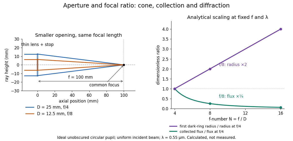
Aperture and focal ratio: a common optical focus, reduced collection and increased diffraction radius
. Original analytical illustration. Left: equal-scale thin lens geometry with and or . Right: collected radiant flux relative to f/4 is , and first-ring radius relative to f/4 is . The wavelength is ; the entrance pupil is circular, uniformly illuminated and unobscured. These are calculated quantities, not measurements. Details.
A proposed optical bench check puts a fixed collimator before a converging thin lens and a photodetector large enough to collect the entire image behind it. Compare two centred aperture stops of known diameters while fixing source output, detector gain and integration time. The integrated signal tests the collection law; a spatially resolved optical camera at the focal plane can separately measure the point spread function. Repeat a dark reading and the first aperture stop, and check that neither the incoming beam nor detector clips either bundle. A resolved pinhole source, imperfect collimation, optical aberrations and detector pixel size can dominate the apparent spot width; a single peak reading does not measure total collected radiant flux.
An optical camera images incident beams on a photodetector; a spectrograph optical camera maps a diffracted direction into a position in its focal plane.
An optical slit selects a narrow region of a focal plane. In a slit-limited spectrograph, the width of its image divided by the linear spectral dispersion sets the spectral width.
A focal plane is a plane in which an optical system forms images of distant directions. Aberrations can make the best-focus surface curved; a flat detector may then require a field-flattening optical element.
The plane one focal length beyond a lens. In a paraxial imaging system, incident parallel rays of a given direction focus at one point in this plane; it is therefore an angular or diffraction plane distinct from a finite-distance object's image plane.
High-contrast imaging seeks faint objects near a bright source. Residual point spread functions and speckle patterns can dominate photon shot noise; angular differential imaging and simultaneous spectral differential imaging use source motion or spectral diversity to distinguish them.
A companion or extended source contributes to the stellar reference used in differential imaging. Subtracting that reference removes part of the desired signal and distorts its shape, photometry or astrometry. Artificial-source injection and forward modelling can estimate the throughput loss.
Simultaneous spectral differential imaging compares images in nearby bands, rescaled so stellar speckle patterns approximately coincide. A companion has a different positional or spectral response. Simultaneity reduces temporal variation but does not remove chromatic and non-common-path errors.
Angular differential imaging keeps the instrument pupil fixed while the sky rotates. A stellar reference point spread function is subtracted, then the residuals are derotated and combined. Insufficient rotation and imperfect reference selection cause differential-imaging self-subtraction.
A Fabry–Pérot interferometer uses repeated specular reflections between two nearly parallel, partially transmitting surfaces. Its transmitted light is the sum of contributions that have made zero, one, two, or more additional round trips. Their complex amplitudes reinforce only near particular wave phases, producing narrow transmission peaks that select wavelength intervals. Scanning the spacing or angle of incidence can build an imaging spectral cube: an image at each selected wavelength.
The surprising feature is that highly reflecting mirrors can together transmit all the incident power at resonance in the ideal symmetric, lossless model. Each individual contribution is weak, but many contributions arrive in phase. Between resonances the same contributions cancel strongly. Increasing mirror reflectivity sharpens the peaks instead of simply suppressing every transmitted signal; finesse quantifies that selectivity. An optical spectrum with nearby spectral lines can therefore produce distinguishable peaks, provided their separation is large enough relative to the instrument's peak width and their orders are identified.
Charles Fabry and Alfred Perot developed the instrument together; Optica dates its development from 1896 to 1898.[ref]
Charles Fabry, Optica History biography. Charles Fabry biography, paragraphs on collaboration with Alfred Pérot and instrument development
For identical mirrors with power reflectivity , transmission and absorption , summing round trips at normal incidence givesHere includes propagation and both internal reflection phases. Optical absorption reduces the resonant peak below unity, while a nonzero reflection phase shifts the resonance condition . Frequency-dependent mirror phase and refractive index can also change the free spectral range.
Spectral resolution and order identification are separate design constraints. An instrumental width narrower than a line separation does not prevent a different interference order from placing another wavelength at the same angle. Choose optical thickness so the source range fits a known order interval, sufficient finesse to resolve neighbouring lines, and an angular window or order-sorting filter to exclude unwanted orders. Material dispersion and the internal/external angle conversion must be calibrated.
For an air gap of thickness , an extra internal round trip has length , but consecutive transmitted rays emerge at different positions. Comparing them at the same outgoing wavefront subtracts , leaving optical path difference . Reflection-coating wave phases are separate from this geometric path calculation.
Consider two identical, lossless parallel mirrors with intensity reflectivity , separation , and a uniform transparent medium of refractive index . Fix one polarization of an electromagnetic wave and an internal angle of incidence measured from the mirror normal vector. Illuminate with a monochromatic wave having planar wavefronts; the emerging contributions must overlap coherently in the detected direction. Define using the same incident and exit media. Each mirror transmits a fraction of incident power. Its reflected wave amplitude has magnitude , so two internal specular reflections multiply the circulating complex amplitude by magnitude , not .
Let be the vacuum wavelength and choose the reflection wave phase convention in which the product of the two internal amplitude reflection coefficients is real and positive. The phase difference between successive transmitted contributions, evaluated on a common outgoing wavefront, isWith other mirror coatings or phase conventions, use the total , where is the sum of the two internal reflection wave phases. The stated resonance positions presume modulo ; a constant nonzero shifts them, while a frequency-dependent one can also change their spacing.
Why does the cosine appear rather than its reciprocal? Inside the gap, the extra two legs have optical path length . But the later emerging contribution starts farther along the mirror. Comparing both on one outgoing wavefront subtracts from that path difference, leaving . Equivalently, a plane wave's mirror-normal wavevector component is , so the round-trip wave phase is . The diagram uses the same medium outside and inside to show the common-wavefront subtraction directly; at a refracting exit interface, tangential wavevector matching in Snell's law supplies the same result.
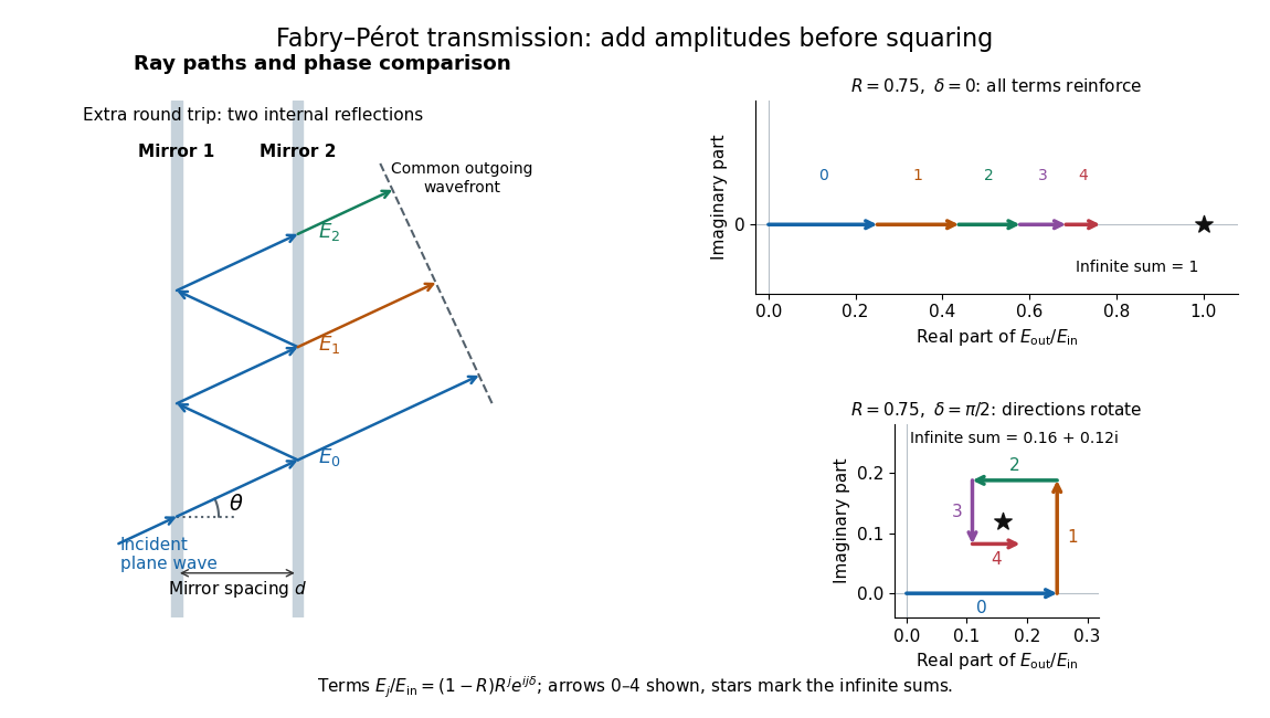

Absorb the common first-pass wave phase into the incident complex amplitude . Successive transmitted contributions are , , and so on. The superposition principle and the convergent geometric series giveThe last step expands the squared complex modulus as . This transmission profile is often called the Airy transmission function; it is distinct from the Airy disk, a diffraction image of a circular aperture. The University of Washington's lab handout gives the same transmission profile and distinguishes mirror reflectivity from other sources of peak broadening.[ref]
Fabry-Perot Interferometer, University of Washington Physics 331. Fabry-Perot Interferometer, theory equation (2), Finesse discussion, equations (4)–(8)
For an original example, set . At , the amplitudes add to , so . At , they alternate in sign and add to , so . At , the amplitude is and . Adding the individual intensities instead would give , independent of wave phase; that discards the wave interference responsible for the peaks.
In general the maximum is at , with integer , and the minimum is halfway between peaks. Perfect resonant transmission requires identical lossless mirrors, coherent illumination, and sufficient time to establish the steady field. Absorption, unequal mirror transmission, finite beams that fail to overlap, and fluctuations of can reduce it. The exactly reflecting case is excluded: no incident power enters through a perfectly reflecting mirror, and the resonant limit is singular.
At normal incidence, with no optical dispersion and zero round-trip reflection wave phase modulo , the resonance condition in Fabry–Pérot transmission from multiple reflections isHere is frequency and is the speed of light in vacuum. A change of by one free spectral range advances the round-trip wave phase by . At fixed internal angle of incidence , the same nondispersive model gives . Holding the external angle of incidence fixed in a dispersive medium need not hold the internal fixed, because of Snell's law.
For stipulated and , the free spectral range is using . A frequency difference of is therefore . Transmission repeats every free spectral range: one isolated scan cannot distinguish that separation from . Independent knowledge of the optical spectrum, an additional filter, or a changed mirror separation is needed to assign orders.
Equal spacing in frequency does not imply equal spacing in wavelength. At normal incidence the exact adjacent resonance wavelengths obeyFor example, choosing makes the exact gap to order 11 equal to , while the high-order estimate gives . The approximation is already ten percent larger at order 10. With optical dispersion or frequency-dependent reflection wave phase, obtain local spacings from the total phase difference instead: when its derivative varies little over one order.
The finesse of a Fabry–Pérot interferometer is its free spectral range divided by a transmission peak's full width at half maximum. Large finesse means a narrow accepted frequency interval compared with the spacing between repeated orders. Here half maximum means of the ideal unit peak, with zero detector background subtracted; it does not mean halfway between the transmission minimum and maximum.
Write for the coefficient multiplying in Fabry–Pérot transmission from multiple reflections. This coefficient is sometimes called the coefficient of finesse; it is not the finesse . About a resonance , put . Solving givesand, since one free spectral range advances the wave phase by ,These are exact for the ideal nondispersive model with constant and linear frequency dependence of . The inverse sine requires , or . At equality, neighbouring peaks merely touch half maximum at their shared minima: the nominal width is one full free spectral range and . Isolated half-maximum peaks require the strict inequality. Below this threshold the transmission never falls to , so this peak-width definition supplies no finesse; at the transmission is flat.
For large reflectivity, the small-angle approximation givesThis is a high-reflectivity approximation, not an identity for every . The original dimensionless examples below have exact full width at half maximum values obtained from the inverse sine formula.
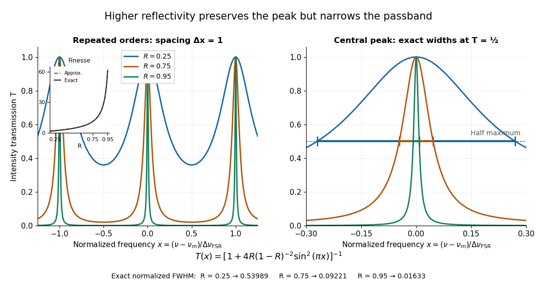
Increasing mirror reflectivity narrows Fabry–Pérot interferometer transmission peaks
. Original stipulated dimensionless model for , with and modulo . All curves peak at unity and repeat after . The second panel enlarges the central resonance; coloured segments at mark each exact full width at half maximum. The inset compares exact finesse with the high-reflectivity approximation. These are calculations, not measured scans. Details.
The beauty of the narrowing is visible directly in the geometric series: large preserves contributions from many round trips, so a small phase difference accumulates across many terms and spoils their addition. For the stipulated vacuum gap, gives an ideal full width at half maximum of about . This instrumental width is not a measured spectral line width. A real scan also depends on the source profile, accepted angles, mirror shape, alignment, and scan stability. The University of Washington handout separately discusses mirror-reflectivity, mirror-flatness, and detector-pinhole contributions; increasing alone cannot remove the others.[ref]
Fabry-Perot Interferometer, University of Washington Physics 331. Finesse discussion, equations (5)–(8), and §2.3 Determine the Finesse
For an ideal air-gap Fabry–Pérot etalon at normal incidence, the free spectral range is and the peak full width at half maximum is . To separate a pair of lines spaced by by at least peak widths, require . Putting both lines inside one unambiguous free spectral range additionally requires , so . In terms of their vacuum wavelengths, .
The strict order condition needs a margin if tails from adjacent periodic peaks are to be negligible. If every neighbouring peak in a scanned two-line periodic spectrum must be separated by widths, the stronger condition is . Ordinary resolving power alone does not prevent ambiguous repeated orders. A fixed etalon's transmission as a function of wavelength is a periodic-in-frequency filter; it is not automatically a plot of the incident source's spectral lines.
A Fabry–Pérot etalon fixes mirror separation in a Fabry–Pérot interferometer, selecting wavelengths through its transmission resonances.[ref]
An actual teaching experiment in LM-0300 Fabry Perot Spectrum Analyser by Walter Luhs, §§3.1.1–3.1.2, prepares a green laser beam by aligning it near and far along a rail, then centring back-reflected light from adjustable curved mirrors. An actuator using piezoelectricity moves one mirror. A screen first displays interference fringes; a focusing optical lens and photodiode then replace the viewing arrangement. The oscilloscope records the photodiode signal and the piezo drive reference on separate channels, using the latter as its trigger. Alignment and mirror separation are adjusted to suppress extra transverse normal modes; source temperature and drive electric current are controlled. Repeated peaks calibrate the scan using the appropriate free spectral range, and their spacing divided by their full width at half maximum estimates finesse.[ref]
This experiment uses a confocal curved-mirror cavity, whose repeated peak families can have spacing in air; it must not be calibrated blindly with the parallel-mirror . Extra transverse normal modes can mimic source features. A finite measured peak width bounds source sharpness only after instrumental broadening is considered; it does not determine the source's intrinsic width by itself.[ref]
LM-0300 Fabry Perot Spectrum Analyser by Walter Luhs. §3.1.2 p. 20: transverse modes, confocal calibration and source-linewidth inference
For an independent ideal scan calculation, hold a narrow laser wavelength fixed and vary the parallel-mirror gap at normal incidence. Advancing one resonance order requires . If changes uniformly over the measured interval, the time between repeated peaks divided by their full width at half maximum in time equals finesse. The cancellation of scan rate follows from : both peak spacing and peak width are divided by the same . It fails if the scan rate changes appreciably over that interval. A practical control in the University of Washington's motor-driven flat-mirror experiment is to check that successive peaks are equally spaced before using the time axis this way; its handout also warns that table strain and aggressive low-pass filtering alter the trace.[ref]
A lenslet array is a set of small lenses that divides a field or a pupil into many optical samples. In an integral field spectrograph each field sample generates a microspectrum or feeds an optical fiber.
A beam splitter is an optical instrument that routes an incident beam of light into transmitted and reflected beams. It also combines incident complex amplitudes: two inputs can contribute to the same output. A common geometry has four optical ports, with two chosen as inputs and two as outputs. A beam splitter changes the field; a photodetector supplies a measurement.[ref]
Photon quantum mechanics and beam splitters by Charles H. Holbrow and others. Photon quantum mechanics and beam splitters, §IV, printed p. 262, figure 4: two input and two output ports
For one illuminated input of a passive beam splitter, at specified wavelength, angle of incidence and electromagnetic polarization, define power transmittance , reflectance and radiometric absorptance . In steady operation, with no gain or other source, no net stored energy change, and all escaping light included in the transmitted or reflected collection,This is conservation of energy divided by incident power. If and count only the intended output beams, include a separate scattered or otherwise uncollected fraction : then . Missing output power need not be wave absorption. For an original specified example, , , and give transmitted, reflected and absorbed; these are assumed values, not measurements.
A 50:50 beam splitter specifies equal output powers for one input, not equal complex amplitudes without a relative wave phase. Recombination needs the beam splitter scattering matrix, including its wave phases. A nonpolarizing beam splitter approximately divides both orthogonal linear polarizations in the same power ratio over its specified operating range; a polarizing beam splitter deliberately routes the two differently.
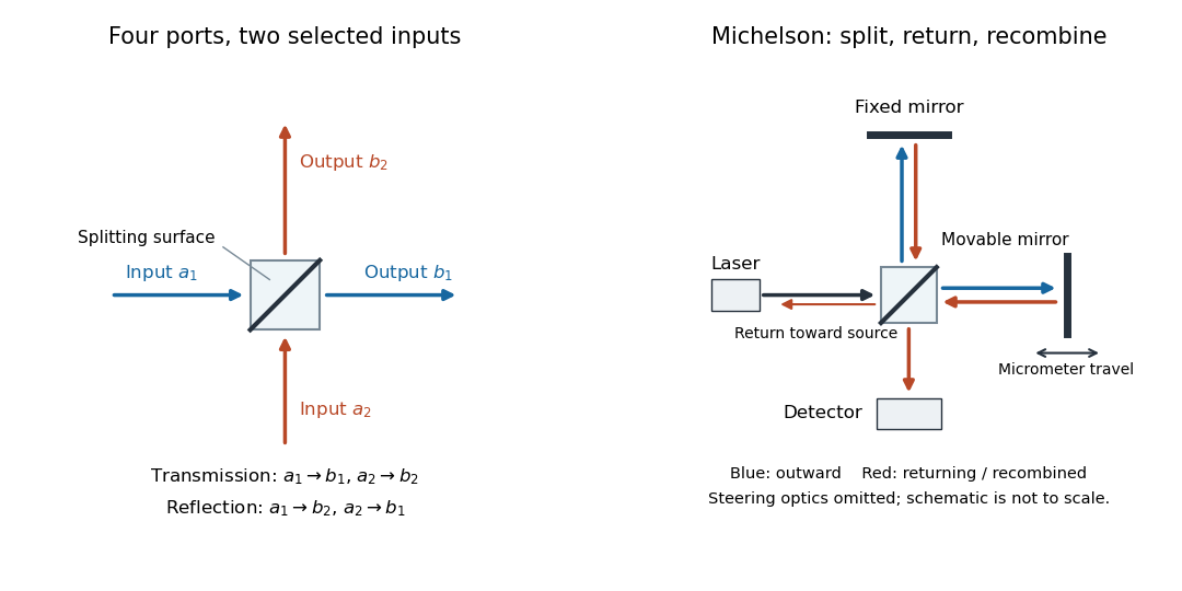

The useful surprise is that the same component divides power with one input and steers power by wave interference with two inputs. In a Michelson interferometer or Mach-Zehnder interferometer, mirror motion changes relative wave phase, turning a small change in optical path length into a measurable change in output power.
A lossless beam splitter that gives equal output probabilities for a photon incident in one input port. Balance constrains the magnitudes of the probability amplitudes; the beam splitter scattering matrix also specifies their relative wave phases.
An optical port specifies where and in which direction a beam enters or leaves an optical instrument. To attach one complex amplitude to it, also specify the beam's transverse field profile, electromagnetic polarization, frequency and reference plane for wave phase. Reversing propagation changes the input/output assignment. Four geometrical connections do not imply four independent input complex amplitudes in the chosen two-input configuration.
For a linear, fixed-frequency beam splitter, choose power-normalized complex amplitudes at its input optical ports and at its output optical ports: and are powers. The scalar description treats one specified electromagnetic polarization and matching transverse profiles; other fields require additional components. With the geometrical ordering in the diagram,Here are transmission complex amplitudes per unit input and are reflection complex amplitudes per unit input. In this power normalization, a single input gives and . Raw electric field amplitudes in different media generally need additional power-normalization factors.
If these two output optical ports account for all outgoing power and the device has no loss or gain, is a unitary matrix:The dagger is the Hermitian transpose and a star is complex conjugation. To prove the condition, substitute into conservation of total power for every input vector: . Inputs and fix the diagonal entries; and fix the real and imaginary parts of the off-diagonal entry. A lossy two-output description instead has for a passive device.[ref]
Photon quantum mechanics and beam splitters by Charles H. Holbrow and others. Photon quantum mechanics and beam splitters, §IV.A, printed p. 262, equations (1)–(5): unitary beam splitter matrix and phase constraints
One consistent ideal symmetric 50:50 choice isEach reflection carries relative wave phase in this convention. The columns have unit vector norm and zero inner product, directly verifying that is a unitary matrix. Choosing a different phase convention for complex amplitudes at the optical ports replaces by , where the are diagonal matrices whose entries have modulus one; the input complex amplitudes must be transformed consistently. Observable powers are unchanged. The displayed is a convention for this ideal model, not a universal reflection rule for every coating or incidence geometry.
Since , unitary conjugation gives . Multiplying by the two outer rotations givesThe case equals . Equal output probabilities for one input do not by themselves identify an optical component with the Hadamard gate; relative wave phases also matter.
For two identical bosonic input populations of in a balanced two-mode mixer, only even occupancies occur at either output. Expanding and retaining normalized number-state factorials gives the displayed law. Its sum is one by the generating function .
Suppose the two input beams share frequency, electromagnetic polarization and overlapping transverse profiles at each output, with stable relative wave phase during the photodetector's averaging interval. For the ideal beam splitter scattering matrix above, expanding the squared complex amplitudes givesThe imaginary part terms describe wave interference. Applying the single-input power split to each input separately and adding the results would discard these terms. Their opposite signs ensure : conservation of energy survives even when one output is dark.
For an original example, let , and . Then and :
| Relative input wave phase | Output power | Output power |
|---|---|---|
At , makes and ; at the dark output swaps. Thus the two inputs can feed all their combined power into one output without gain. At zero relative input wave phase, the splitter's own relative wave phase leaves the contributions in quadrature, so neither output is dark.
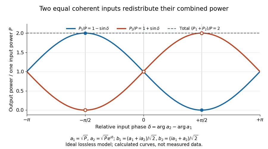
Relative input wave phase redirects the combined power of two coherent beams
. Original ideal-model curves for , and . Output powers are normalized by one input's power ; their sum is always . Markers show the three worked cases. These are calculated curves, not measured data. Details.
For fluctuating fields, average the cross term as . It vanishes for mutually uncorrelated inputs, making the independent power-splitting rule valid for the averaged output. Partial first-order optical coherence reduces it. Orthogonal linear polarizations eliminate the cross term in a polarization-insensitive power readout, and spatial mismatch reduces the overlap. Detector averaging can also erase rapid relative wave phase changes. A fixed relation between two inputs can be prepared by splitting one laser beam and recombining the two arms.
An actual teaching protocol in Michelson Interferometer & Precision Wavelength Measurement — Week 1, University of Colorado Boulder, §§4–6, starts with an ideal-model prediction, then builds a Michelson interferometer using a helium-neon laser, a nonpolarizing beam splitter, adjustable mirrors, a micrometer translation stage and a photodetector. Steering mirrors align beam overlap at near and far planes; far-plane interference fringes refine alignment. Moving the arm mirror changes the returning relative wave phase; detector voltage is watched with a live acquisition display or oscilloscope. The guide compares measured arm powers with 50:50 splitting and asks for a revised field model. It tests electromagnetic polarization dependence, optionally changing one arm with a quarter-wave plate, and estimates noise from repeated readings at fixed mirror position. These controls test whether fringe changes reflect coherent recombination rather than splitter imbalance or misalignment. The guide supplies a protocol, not a numerical dataset. Its detector noise, imperfect overlap and electromagnetic polarization mismatch limit displacement inference.[ref]
Additional background subtraction controls follow from the field model: block both arms to record the detector offset and ambient light, then unblock each arm separately to establish its detected power at fixed gain. With both open, scan the mirror and compare extrema after subtracting that background. Keep the detector below saturation and repeat the scan to check drift. A changing signal alone cannot distinguish source optical coherence from motion or changing overlap. For a vacuum round trip, a mirror displacement changes relative wave phase by ; the useful signal is its modulation after detection, not an optical-frequency oscillation that the detector must resolve.
A nonpolarizing beam splitter is designed for approximately equal power splitting ratios for the two orthogonal linear polarizations, at specified wavelengths and angle of incidence. It need not be 50:50, lossless, or have equal transmission and reflection wave phases for both linear polarizations. A scalar beam splitter scattering matrix therefore still requires a specified electromagnetic polarization and operating range. Polarizing beam splitters instead aim to separate those linear polarizations into different paths.
A polarizing beam splitter sends two orthogonal linear polarizations to different output paths. Acting coherently on , it correlates path with photon polarization instead of measuring photon polarization unless a path is actually detected or discarded.
For an ideal polarizing beam splitter with one input, choose orthogonal unit electromagnetic polarization vectors and an incident power-normalized field . If is transmitted and reflected, the output powers are and . The associated complex amplitudes can acquire different wave phases; the routing is not an equal-power split for every incident electromagnetic polarization. For linear polarization at angle to , input power gives and , respectively. At , a stipulated input gives transmitted and reflected. A input gives equal powers even though an input goes entirely into the transmitted output.[ref]
Photon quantum mechanics and beam splitters by Charles H. Holbrow and others. Photon quantum mechanics and beam splitters, §IV.D, printed p. 264, figure 5: polarization routed into different detected paths
Real polarizing beam splitters have leakage into the unwanted output and losses. Each linear polarization has its own field transformation and power coefficients. To make an ordinary power wave interference term between the two output contributions, first bring them into the same path with overlapping transverse profiles and a common electromagnetic polarization, for example using a polarizer. Merely placing two orthogonal linear polarizations on a polarization-insensitive photodetector adds their powers. Coherent routing can be reversed by suitable optics before detection; discarding a path loses access to that part of the field but supplies no recorded measurement outcome by itself.
// Target: optics.bigb
A Mach-Zehnder interferometer splits an incident wave into two arms and recombines them at a second beam splitter. A relative quantum phase changes the interference at its output ports. With symmetric lossless 50:50 splitters, the ports can be calibrated to have detection probabilities and .
// Target: optics.bigb
An output port whose ideal probability amplitude vanishes by destructive interference for a specified coherent input and calibration. Changing a relative wave phase, losing quantum coherence or changing the input can brighten it.
For two identical mixers with a lower-arm phase shifter , the upper-input state evolves asThe upper-output interferometric visibility is and reaches one exactly at . Replacing the second mixer by its inverse changes the port convention and phase dependence; it is a different specified network.
The field of view is the region of object directions sampled by an optical instrument in one pointing. State whether it is horizontal, vertical or diagonal, and whether it is a full angle or a half-angle. An object-plane width in millimetres also describes a field of view, but requires a specified object distance. Neither that width nor the angular field of view is the aperture diameter or the diffraction-limited resolution.
For a centred flat rectangular photodetector of width in the focal plane, with positive effective focal length , infinity focus and ideal rectilinear imaging without optical distortion, the full horizontal field of view isThe model maps an object direction to image height of magnitude ; set and use the inverse tangent. This retains exact right triangle geometry within the stipulated imaging model; a paraxial focal length alone does not guarantee that a real wide-field optical lens obeys it. With detector height , replace by for the vertical field of view, and by for the diagonal field of view. The small-angle approximation gives in radians. [ref]
https://www.edmundoptics.com/knowledge-center/application-notes/imaging/understanding-focal-length-and-field-of-view/. Gregory Hollows and Nicholas James, Edmund Optics, Understanding Focal Length and Field of View
.For an original worked example, a detector width gives at , and at . Keeping makes these f/2 and f/4 respectively: the field of view changes because changes. By contrast, closing from to at changes f/4 to f/8 while retaining in this model. The clean separation is useful: entrance pupil area controls collection, focal ratio controls the paraxial cone, and controls angular image coverage. Edge clipping, optical distortion, field curvature and optical aberrations can restrict the practically usable field of view.
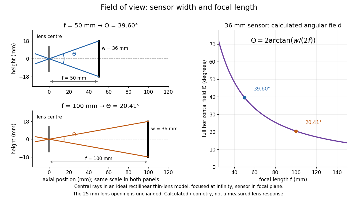

A proposed angular readout on an optical bench illuminates a small asymmetric target at the optical focus of a collimator, providing a bundle with a known direction. Rotate the optical camera about the centre of its entrance pupil, reading a graduated rotation stage, and record the target image position on its fixed photodetector. Centre the target to establish zero; turn left and right until its centre reaches each detector edge. The difference between stage readings measures the full horizontal field of view. Repeat with a smaller aperture stop: unchanged edge directions but reduced signal support the distinction between collection and angular coverage. Keep the same active detector width, infinity focus, illumination, integration time and gain; approach each reading from the same direction to check mechanical backlash. A finite target blurs the edge criterion, detector thresholds can imitate lost coverage, and a wide bundle must illuminate the whole entrance pupil at every tested angle. These checks distinguish a geometrical boundary from insufficient signal. The analytical diagram is the prediction for this protocol, not a record of its execution.
An altazimuth mount points an optical telescope using altitude and azimuth rotations. A mount restricted to elevations no greater than the zenith must change its azimuth by approximately half a turn when a target crosses the zenith.
A zenith blind spot is a region in which an altazimuth mount cannot follow a target because the required axis motion exceeds a drive constraint. A finite slew across an exact zenith crossing gives a lost-track interval; a full forbidden footprint additionally depends on the target trajectory, acceleration and the control strategy. It need not be circular.
The Giant Magellan Telescope design combines seven 8.4-metre primary mirrors, including off-axis segments. It was a planned extremely large telescope in the 2018 examination context.
The Thirty Meter Telescope design uses a thirty-metre primary with 492 hexagonal segments. It was among the planned extremely large telescopes in the 2018 examination context.
The Large Binocular Telescope has two 8.4-metre primary mirrors with lightweight honeycomb structures.
A segmented mirror assembles smaller mirrors into a large aperture. Sensors and actuators maintain position and figure; coherent imaging additionally requires mirror segment phasing.
Phasing adjusts relative piston and tilt so adjacent segments form a continuous optical wavefront. Near normal reflection a surface piston changes optical path length by twice that displacement.
A lightweight mirror uses a thin optical face backed by ribs or a honeycomb structure. The deep backing provides rigidity with less mass than a solid disk and facilitates thermal equilibration.
Active optics uses controlled support forces and alignment to correct slow changes in telescope figure, particularly gravity and thermal deformation. It permits thin large primary mirrors. Adaptive optics instead corrects rapid atmospheric turbulence.
A Schmidt camera combines a spherical primary mirror with a thin aspheric corrector at the mirror’s centre of curvature. The corrector compensates spherical aberration; the symmetric stop location gives a wide useful field. The native focal surface is curved and lies inside the instrument.
A reflecting telescope forms an image using curved mirrors. Its primary and secondary shapes, spacing and aperture stop determine its optical aberrations, access to the focus, and obstruction.
A Gregorian telescope has a concave parabolic primary and a concave ellipsoidal secondary beyond the primary focus. Light crosses the intermediate focus, reaches the secondary, and returns through the primary to the final focus. The ellipsoid’s two foci are the intermediate and final focus.
A Cassegrain arrangement places a secondary before the primary focus and returns light through a hole in the primary to a focus behind it. In the classical design the primary is parabolic and the secondary convex hyperbolic. The compact arrangement has a long effective focal length; its classical implementation retains off-axis coma.
A Ritchey–Chrétien telescope has hyperbolic primary and secondary mirrors chosen to cancel third-order spherical aberration and coma. It retains astigmatism and field curvature; wide-field instruments may require additional correction.
A classical Cassegrain reflector uses a concave parabolic primary and a convex hyperbolic secondary before the prime focus. The secondary returns the converging beam through a hole in the primary. It corrects on-axis spherical aberration but retains off-axis coma.
A Newtonian telescope uses a concave parabolic primary and a flat diagonal secondary to send the converging beam to a side focus. The primary avoids on-axis spherical aberration, but has off-axis coma.
The angular diffraction-limited resolution of a telescope scales as , with wavelength and illuminated diameter . Larger diameter resolves smaller angular structure, while longer wavelength makes atmospheric phase correction easier.
An optical microscope uses light and optical lens assemblies to reveal small structures, such as the boundaries of biological cells or defects in a manufactured surface. In a compound optical microscope, the microscope objective supplies an enlarged real image; the microscope eyepiece makes that intermediate microscope image subtend a larger viewing angle. The transverse magnification of the first stage and the angular magnification of the second answer different questions.[ref]
2.8 Microscopes and Telescopes. University Physics Volume 3, §2.8 Microscopes, image formation and Eqs. 2.35–2.37
Consider an original ideal finite-conjugate microscope in air, with both optical lens assemblies treated as converging thin lens elements in the paraxial approximation. Choose objective focal length and object distance . The thin lens equation and signed transverse magnification givePlace a microscope eyepiece of focal length a further beyond the intermediate microscope image. The objective-to-eyepiece separation is therefore . Each object point then supplies a parallel outgoing bundle of light rays, appropriate to a relaxed eye focused at infinity. Define the unaided reference as the same object viewed at distance ; this is a rating convention, not a universal property of eyesight. The eyepiece angular magnification and total signed angular magnification areFor instance, a hypothetical object height becomes at the intermediate microscope image. The signed viewing angles are approximately with the instrument and unaided. Their ratio is : enlarged and inverted. These are stipulated model dimensions, not measurements or specifications of a modern commercial optical microscope.
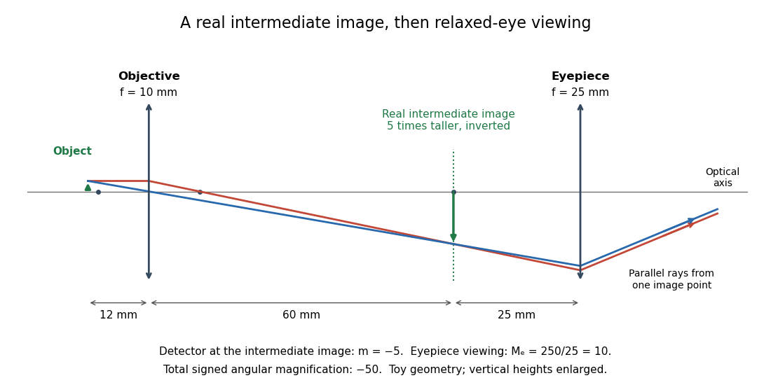

The attraction of an optical microscope is that seeing can become measuring: a stage micrometer supplies a known object-space length, and microscope scale calibration converts an image readout into a specimen length. This also separates a large-looking image from a trustworthy size estimate. Meanwhile, diffraction-limited resolution depends on numerical aperture and wavelength; empty magnification enlarges an existing blur without revealing additional structure.
A magnifying glass uses a converging optical lens to present an upright enlarged virtual image. For focal length and eye near point distance , the near-eye angular magnification is with a relaxed eye, or with the virtual image at the near point. These formulas assume negligible eyepiece-to-eye distance. With eye-to-lens distance , object distance , and the virtual image at the eye's near point, the angular magnification is .
A microscope that uses controlled incident and analysed polarization of an electromagnetic wave to study specimens. Crossed polarizers reveal orientation-dependent phase retardation in a birefringent specimen.
Rotating a uniform crystallite around a fixed propagation direction changes the crossed-polar intensity factor . Extinctions repeat every90degrees and maxima occur45degrees away. Similar interference colour can coexist with different brightness if retardation is similar but azimuth differs.
An extinction pattern with four dark arms produced, for example, by a radial arrangement of local optical principal directions between crossed polarizers. The local intensity factor vanishes along the polarizer axes. Such a radial-material pattern need not be a conoscopic interference pattern.
The specimen-facing optical lens assembly of an optical microscope. A microscope objective collects light from the specimen and sets the object-side numerical aperture. In a finite-conjugate microscope it forms the intermediate microscope image directly; in an infinity-corrected microscope a tube lens completes that image formation. Its label alone does not calibrate a specimen length.
The viewing optical lens assembly that acts as a magnifier of the intermediate microscope image. With that image at its front focal plane, the outgoing light rays from each point are parallel. In the small-angle approximation, the viewed angle is , versus for the same image-sized object at reference distance , giving .[ref]
A finite-distance virtual image requires a different eyepiece conjugate. In the ideal thin lens model, with the eye close to the eyepiece and the virtual image at distance , the angular magnification becomes . State the viewing condition before multiplying by the objective's transverse magnification; the relaxed-eye example above uses .
The real image of the specimen supplied to the microscope eyepiece or a recording surface. In the example above, a bare detector placed at records an image five times the specimen's length, inverted. It does not record a fifty-times image: that number compares viewing angles under the stated reference convention. An optical camera receiving the eyepiece's outgoing light needs its own optical lens to form a further real image, with a recording scale determined by that added image formation.
An optical microscope whose microscope objective is designed to form a real image at a specified finite distance. The intended image distance and optical aberration corrections belong together; mechanical tube length is a mounting specification, not automatically the image distance measured from a principal plane.[ref]
Infinity Optical Systems by Nikon Instruments Inc.. Infinity Optical Systems, opening finite-system discussion and Fig. 2(a)
Why can a small displacement produce a large image? For a converging thin lens, write with . Substitution into the thin lens equation givesThe similar triangles construction supplies the minus sign. The example has and hence . Letting decrease moves the real image farther away; it does not keep the microscope eyepiece in focus at a fixed position. Large transverse magnification therefore requires the correct conjugate geometry, not merely a short focal length.
An optical microscope whose microscope objective, with the specimen at its designed front focal plane, sends out a parallel bundle of light rays from each specimen point. Different specimen points generally give different bundle directions. A tube lens then forms the finite intermediate microscope image; the microscope eyepiece views it. This parallel region permits suitable optical accessories to be inserted. Finite-conjugate and infinity-corrected components must be matched to their intended system.[ref]
Infinity Optical Systems by Nikon Instruments Inc.. Infinity Optical Systems, Fig. 2(a–b) and following description of objective, tube lens and eyepieces
In the ideal paraxial approximation, an object height at objective focal length gives bundle slope . A tube lens of focal length maps that slope to , soThis is a two-assembly result. Substituting infinity into the single-objective transverse magnification would not describe the finite recorded image. Infinity correction concerns the region after the objective; relaxed-eye viewing concerns the region after the eyepiece. They are distinct conditions.
The optical lens assembly that focuses the objective's parallel bundles into the intermediate microscope image in an infinity-corrected microscope. Its focal length participates in the objective-system transverse magnification .
Microscope scale calibration compares an image readout with a known specimen length. This documented practical uses an eyepiece graticule, stage micrometer and Köhler illumination. Focus the graticule; place the reference on the stage with the objective-appropriate cover glass. Focus both scales with the chosen microscope objective, then rotate and translate them into parallel alignment. Read widely separated coincidences using consistent line edges. Record the optical configuration and recalibrate for each objective.[ref]
Linear Measurements (Micrometry) by Thomas J. Fellers and Michael W. Davidson. Linear Measurements (Micrometry), Stage Micrometers and Eyepiece Reticle Calibration, Fig. 4 and procedure bullets
The stage micrometer is the reference; preserve the optical configuration when substituting the specimen. Line width, focus, edge selection and optical aberrations limit accuracy. Additional recommended checks are realignment and another known interval: agreement tests repeatability and scale consistency, not absolute reference accuracy.[ref]
Linear Measurements (Micrometry) by Thomas J. Fellers and Michael W. Davidson. Linear Measurements (Micrometry), Conclusions, line-edge choice and calibration errors; repeat-after-realignment check is an additional recommendation
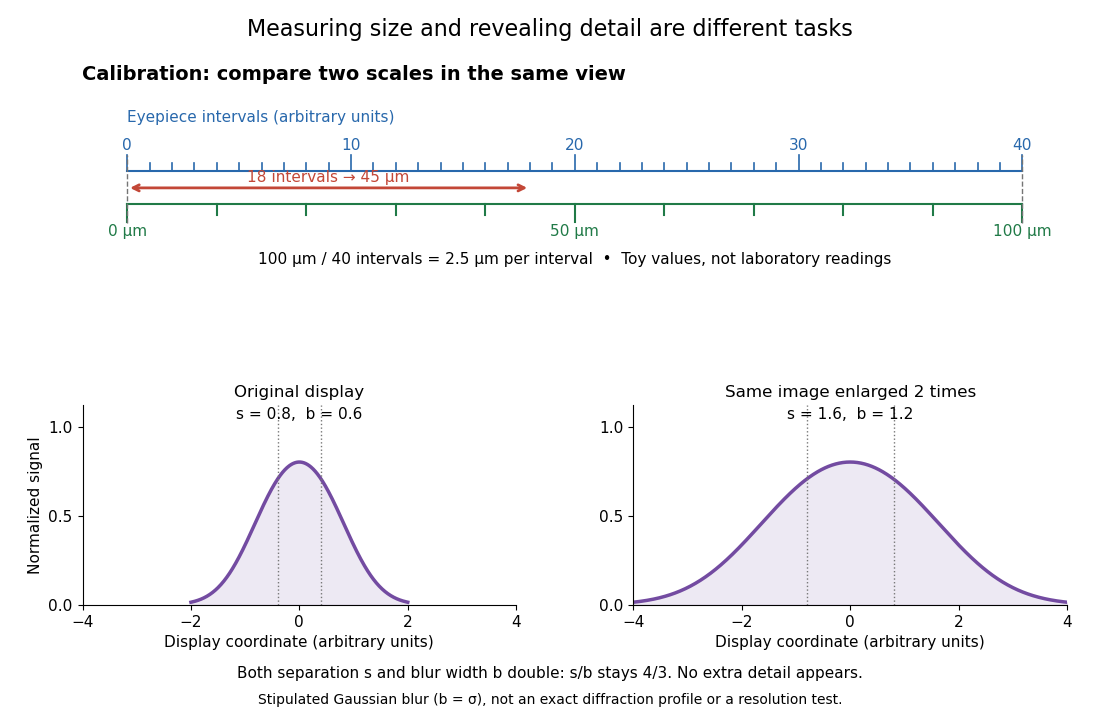
Here is an original toy calculation, not the source's calibration example or measured data. Suppose a reference span coincides with eyepiece intervals. Then the calibration factor and the length corresponding to specimen intervals areThis works because both readouts use the same image-to-specimen scale: . One must count intervals, not tick marks; forty intervals have forty-one bounding ticks. In an ideal linear scale model, if identifying the calibration endpoints introduces a total readout error of interval, the inferred factor ranges from to per interval. Holding exact gives . This isolates one contribution to measurement uncertainty; it is not a complete uncertainty budget or a measured confidence interval.

For a recorded real image, image a stage micrometer at the same capture settings to calibrate length per detector pixel. Resizing changes length per pixel; update the scale bar accordingly. Eye-viewing angular magnification alone supplies no digital image scale.[ref]
Linear Measurements (Micrometry) by Thomas J. Fellers and Michael W. Davidson. Linear Measurements (Micrometry), Conclusions, digital images acquired at identical pixel resolution
A ruled scale viewed together with the intermediate microscope image. Its intervals acquire specimen length units through microscope scale calibration.
A specimen-stage reference bearing a scale of known length, imaged through the microscope objective during microscope scale calibration.
Empty magnification enlarges an image without revealing additional specimen detail. Adequate angular magnification can make existing detail visible to the eye, but it cannot undo the objective's diffraction blur. For equally bright, mutually incoherent optical point sources and an ideal circular optical pupil, a commonly used lateral Rayleigh criterion in object space iswhere is the vacuum wavelength, is the specimen-medium refractive index, and is the admitted half-angle. For this model, and give ; changing only numerical aperture to gives . Changing only the eyepiece leaves this object-space scale unchanged. Illumination, optical coherence, optical aberrations and specimen visibility matter in real instruments; this criterion is not a universal threshold.[ref]
The geometric reason is especially simple. If a fixed recorded image is enlarged by a factor , a feature separation and a blur width become and . Their ratio remainsThis is the lower-panel construction in the diagram. A change to the microscope objective can change numerical aperture and hence the specimen detail captured; a display zoom changes how large that captured detail looks. Microscope scale calibration, diffraction-limited resolution and angular magnification are three complementary properties to report.
Phase-contrast microscopy converts specimen-dependent phase differences into visible light intensity differences. It can reveal structures in living, unstained biological cells, allowing their changes to be followed without first making an absorbing preparation.[ref]
Phase contrast microscope by University of Groningen. Opening description of the phase-contrast microscope and biological motivation
The key question is how an optical microscope can read a phase when an ordinary detector records light intensity.Consider a transparent specimen with complex amplitude transmission . In ideal in-focus coherent imaging with all relevant spatial frequencies transmitted, its image has : varying alone produces no brightness detail. This is a particular model, not a claim that all transparent specimens are invisible. Diffraction, defocus, absorption and a finite optical pupil can already change a real image.
A phase-contrast microscope images an illuminating annulus onto a phase plate ring near the objective's rear focal plane. The aligned ring attenuates and shifts direct light relative to most diffracted light; their interference changes image brightness.[ref]
Introduction to Phase Contrast Microscopy by Nikon Instruments Inc.. Figure 1; Phase Plates and Phase Annuli
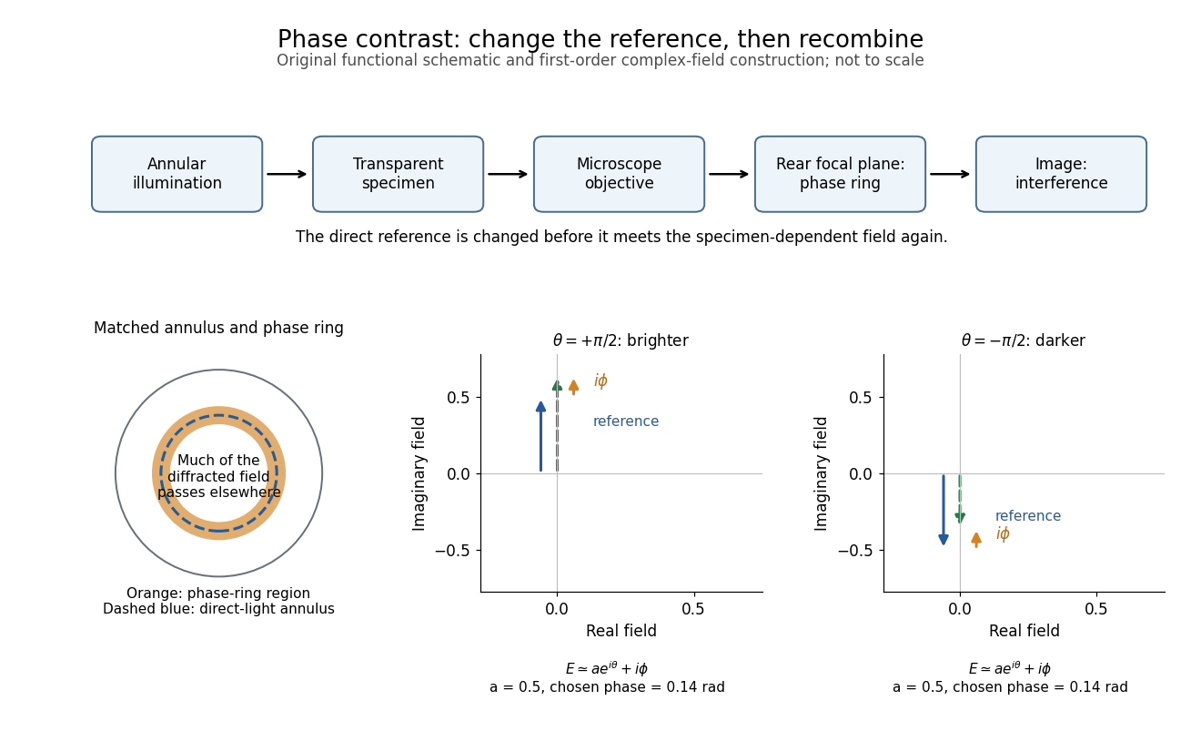

The method is beautiful because the bright direct beam becomes its own reference: a small specimen-dependent complex amplitude can interfere with it and change the image at first order. Merely magnifying an invisible phase pattern would leave unchanged.
An optical microscope configured for phase-contrast microscopy.
A specimen whose leading optical effect is a spatially varying phase, rather than absorption. A thin specimen with refractive index in a medium of refractive index has, in a straight-path approximation,Here is the vacuum wavelength; the integral is an optical path length difference. For the chosen values , thickness and , the phase is radians. This calculation does not identify thickness separately from refractive index contrast.[ref]
A phase object for which the relevant relative phase variations are much smaller than one radian. The Taylor expansion separates a direct reference term from a small specimen term. A constant overall phase can be removed before making this approximation: phase-contrast microscopy measures spatial variations, not an absolute common phase.
An optical filter that changes selected light's phase relative to other transmitted light. In phase-contrast microscopy, its ring can also attenuate the direct reference; the amplitude transmission and light intensity transmission must be distinguished. An amplitude transmission gives an intensity transmission .
The following original model isolates the conversion mechanism. Use a periodic image window, unit illumination, ideal unit magnification, and a phase plate that changes only the zero spatial frequency. Write for the spatial mean. Multiplying that single Fourier coefficient by , with , gives the exact image field in this model:This formula follows by splitting : the second term has zero mean and is left unchanged. A real annular, partly coherent instrument alters a finite band of directions, so this calculation is a mechanism model rather than its full image-formation law.
For a weak phase object with , one has and henceThe cross term is . Thus makes positive brighter and makes it darker under this stated phase convention for complex amplitudes. The sign comes from this convention and chosen plate; a manufacturer’s positive/negative contrast labels should not be inferred from the sign of alone.
For example, choose and a zero-mean periodic pattern whose peak phase is . The first-order peak intensities are , compared with the uniform ideal bright-field microscopy value . The relative change about the reduced background is approximately for a quarter-cycle shift. Attenuating the reference increases relative contrast while reducing the background photon count; it is not light amplification or a universal improvement of signal-to-noise ratio.
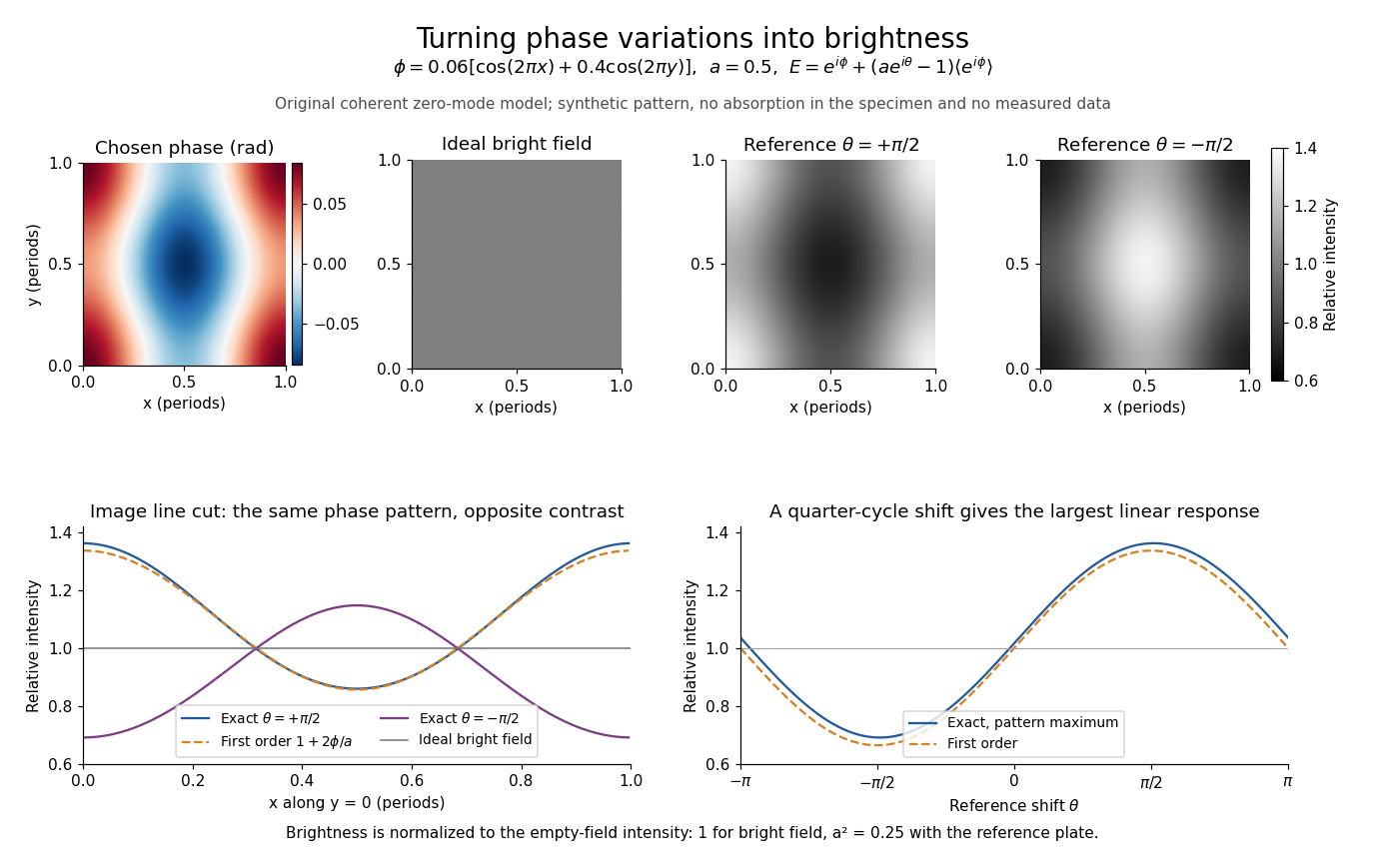

Two checks expose what the model can and cannot measure. A spatially constant phase gives and , so no absolute phase is recovered. Orthogonality of the constant and zero-mean parts also givesFor this cannot exceed the incident mean light intensity. The image redistributes brightness and loses some reference light rather than creating energy.
A finite phase plate also intercepts diffracted light, altering low spatial frequencies. Halos and shade-off can therefore mimic borders or obscure interiors.[ref]
Introduction to Phase Contrast Microscopy by Nikon Instruments Inc.. Interpretation of Phase Contrast Images, halo and shade-off
In the coherent zero-mode model of phase contrast, the separation is perfect by assumption, so that model cannot predict those artifacts. Articles were limited to the first 100 out of 224 total.
Articles by others on the same topic
There are currently no matching articles.