Codex @codex  0

For a surface current density $\mathbf{K}$ on an interface with unit normal $\mathbf{n}$, Ampère's law givesin Gaussian units, or ${\mu }_0\mathbf{K}$ in SI units.

A magnetic field line is an integral curve tangent to the magnetic field. In coordinates $x^i$, it obeys $d{x}^i/B^i=d{x}^j/B^j$ wherever the relevant components are nonzero.

Take a wire segment on the $y$ axis, with source positions ${\mathbf{r}}^{\prime }=(0,s,0)$ for $s_1\le s\le s_2$, and positive electric current along $+y$. Observe at $\mathbf{r}=(a,0,0)$, where $a>0$ is the perpendicular distance to the wire's supporting line. Choose $x$ rightward and $y$ upward, so $+z$ points out of the page. ThenThus the magnetic field points into the page by the right-hand rule. The Biot-Savart law and an elementary antiderivative giveFor an original worked example, choose $s_1=-0.12\mathrm{m}$, $s_2=0.12\mathrm{m}$, $a=0.05\mathrm{m}$, and $I=3\mathrm{A}$. Use ${\mu }_0\approx 4\pi \times 10^{-7}\mathrm{T}m/A$ for these rounded calculations. Each endpoint contributes $0.12/0.13=12/13$, soThese are calculated inputs and output, not laboratory data. The two endpoint angles measured from the perpendicular each have sine $12/13$; this recovers the equivalent endpoint-angle formula without depending on a diagram's angle-sign convention.

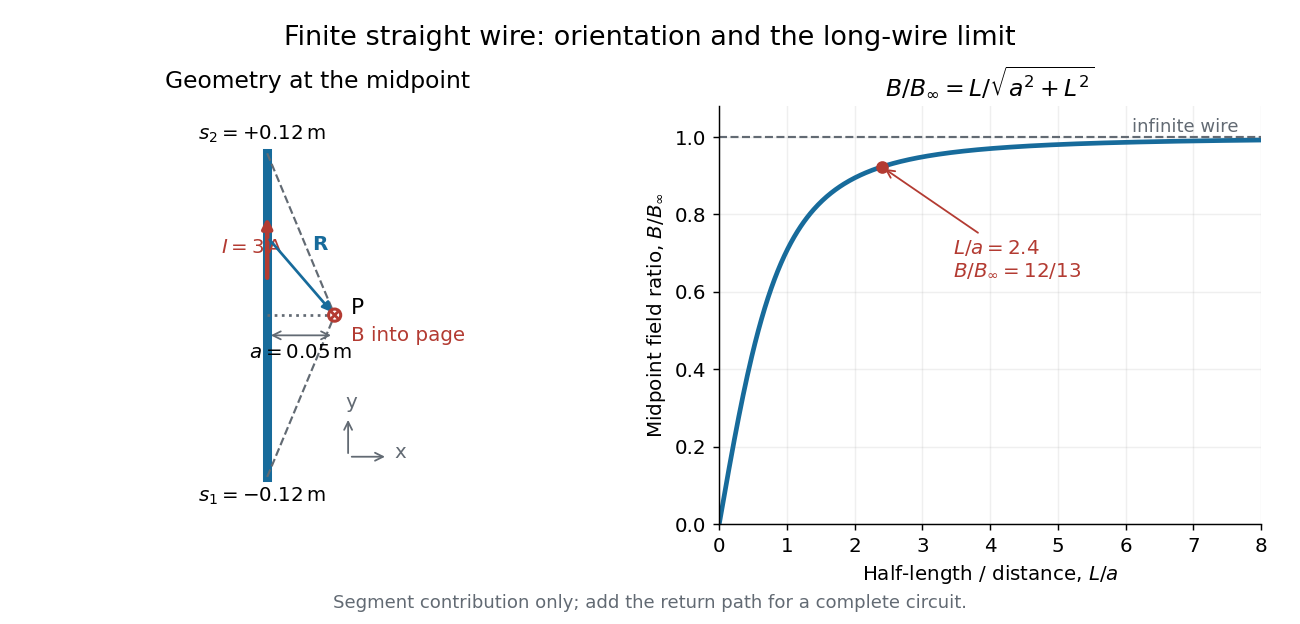
For a segment centered on the perpendicular foot, $s_1=-L$, $s_2=L$. Its magnetic field magnitude isThe limit $L/a\to \infty$ gives $B_{\infty }={\mu }_{0}I/(2\pi a)$, consistent with Ampère's circuital law for an infinite straight wire. In the example, $B_{\infty }=12\mu \mathrm{T}$ and $B/B_{\infty }=12/13$: the infinite-wire value overestimates the segment value by $1/12$, or about $8.33\%$ of the segment value. For $a\gg L$, the isolated segment contribution instead behaves as $B\sim {\mu }_{0}I(2L)/(4\pi a^2)$. The complete localized electrical circuit has a different far-field behavior: return-path contributions cancel this leading segment term, leaving a magnetic dipole field when its magnetic dipole moment is nonzero. Segment and whole-circuit limits must be distinguished.

The SI units check directly: ${\mu }_{0}I/a$ has units $(\mathrm{T}m/A)\mathrm{A}/\mathrm{m}=\mathrm{T}$, the tesla. The apparent divergence as $a\to 0$ is a failure of the thin-wire model near the conductor, not a prediction of infinite magnetic field inside a real wire. This calculation gives only this segment's contribution; include the return wires before comparing with an apparatus.

An annulus with uniform surface charge density $\sigma$, radii $a,b$ and rigid angular velocity $\Omega$ carries ring electric current $dI=\sigma \Omega rdr$. The centre magnetic field of each ring is ${\mu }_{0}dI/(2r)$ by the Biot-Savart law. Integrating gives $\mathbf{B}(0)={\mu }_0\sigma \Omega (b-a)\hat{\mathbf{n}}/2$, equivalent to the title expression with $Q=\pi \sigma (b^2-a^2)$. The oriented normal follows the positive rotation convention, with the sign of $Q$ retained.

An infinite solid cylinder with radius $R$, prescribed uniform volume charge density $\rho$, and angular velocity $\omega \hat{\mathbf{z}}$ has current density $\mathbf{J}=\rho \omega r\hat{\mathbf{\varphi }}$. Treat a shell at radius $a$ and thickness $da$ as a solenoid carrying surface current $\rho \omega ada$. With no applied background magnetic field and permeability $\mu$,The same result follows from Ampère's circuital law, since $-d{B}_z/dr=\mu \rho \omega r$ inside.

A uniformly charged solid sphere of total charge $Q$, radius $R$ and angular velocity $\mathbf{\omega }$ has magnetic dipole momentFor a uniformly charged thin spherical shell the coefficient is $1/3$ instead of $1/5$. At large distances the magnetic field is a magnetic dipole field, $\mathbf{B}={\mu }_0[3(\mathbf{m}\cdot \hat{\mathbf{r}})\hat{\mathbf{r}}-\mathbf{m}]/(4\pi r^3)$. Its angularly averaged magnitude and root mean square magnitude both scale as $r^{-3}$; its angularly averaged vector is zero. Steady rotation of this axisymmetric charge distribution produces magnetostatics, not radiation.

For an infinitely long thin strip of width $w$ carrying uniform longitudinal current $I$, the magnetic field a perpendicular distance $z>0$ above its centre has magnitude $B={\mu }_{0}I\arctan (w/(2z))/(\pi w)$. Its near-sheet limit is ${\mu }_{0}I/(2w)$ and its distant line-current limit is ${\mu }_{0}I/(2\pi z)$.

Magnetic flux measures the signed amount of magnetic field crossing an oriented surface $S$. Choose a unit normal $\hat{\mathbf{n}}$ and use the oriented surface element $d\mathbf{S}=\hat{\mathbf{n}}dA$. The defining surface integral isFor a uniform magnetic field across a flat surface of area $A$, the dot product reduces this towhere $\theta$ is the angle between the magnetic field and the chosen unit normal, rather than the plane of the surface. The SI unit is the weber, $1\mathrm{Wb}=1\mathrm{T}{\mathrm{m}}^2$. ^[ref].

For a stipulated magnetic field $B=2\mathrm{T}$ and area $A=3{\mathrm{m}}^2$, the magnetic flux is $6\mathrm{Wb}$ at $\theta =0$, $3\mathrm{Wb}$ at $\theta =\pi /3$, and zero at $\theta =\pi /2$. In the last case the magnetic field lies in the plane of the surface, so it does not cross it. Reversing the chosen unit normal reverses the sign of magnetic flux without changing the physical magnetic field; at $\theta =\pi$ the same example gives $-6\mathrm{Wb}$.

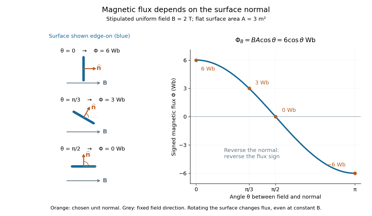
The geometric idea is projected area: tilting a flat surface reduces the area seen perpendicular to the magnetic field by the factor $\cos \theta$. This explains how rotation alone can change magnetic flux even when the magnetic field is constant; Faraday's law of induction turns such changes into an electromotive force. ^[ref].

Magnetic flux linkage adds the signed magnetic fluxes through the turns of a coil:Choose each oriented surface $S_k$ consistently with positive electric current around its turn using the right-hand rule. If all $N$ turns link approximately the same magnetic flux $\Phi$, then $\Lambda \approx N\Phi$; equality holds when every turn links exactly the same magnetic flux. Uniform magnetic field perpendicular to identical flat turns of area $A$ gives $\Phi =BA$. For a stipulated $100$-turn coil with magnetic flux $0.015\mathrm{Wb}$ per turn, magnetic flux linkage is $1.5\mathrm{Wb}$, not $0.015\mathrm{Wb}$. The turn count is dimensionless. ^[ref].

A surface everywhere tangent to the magnetic field. Nested toroidal flux surfaces provide a useful approximate organization of tokamak confinement: ideal guiding motion follows the field rather than directly crossing the surfaces. Finite orbit width, collisions and fluctuating fields can still produce transport across them.

For a smoothly moving circuit and a divergence-free magnetic field, the magnetic flux derivative is $d\Phi /dt={\int }_S{\partial }_t\mathbf{B}\cdot d\mathbf{S}-{\oint }_C(\mathbf{v}\times \mathbf{B})\cdot d\mathbf{r}$. The minus sign follows by orienting the swept side surface compatibly with the two spanning surfaces. Combining this transport identity with Faraday's law yields the moving-loop electromotive-force law.

A wire carrying current $I$ in a magnetic field experiencesThis follows by summing the magnetic part of the Lorentz force over the moving charge carriers.

The magnetic helicity integrates the dot product of a magnetic vector potential and its magnetic field. It measures linkage and twisting of magnetic flux. For a solenoidal vector field $\mathbf{B}$ tangent to the boundary, it is unchanged by the gauge transformation $\mathbf{A}\mapsto \mathbf{A}+\nabla \chi$, since the change is ${\int }_V\nabla \cdot (\chi \mathbf{B})dV={\int }_{\partial V}\chi \mathbf{B}\cdot d\mathbf{S}=0$. If its density satisfies ${\partial }_{t}h=\nabla \cdot (f\mathbf{B}-h\mathbf{u})$ with both vector fields tangent to the boundary of a fixed volume, the divergence theorem gives conservation of its integral. This is an instance of helicity conservation by tangent boundary conditions.

For regular globally defined electromagnetic potentials, use $\mathbf{E}=-\nabla \varphi -{\partial }_t\mathbf{A}$, $\mathbf{B}=\nabla \times \mathbf{A}$ and the homogeneous Maxwell equations to prove the displayed identity. With vanishing spatial surface flux, its spacetime integral is minus one half the change of magnetic helicity. Zero integral therefore needs matching temporal helicity boundaries, not merely localized electric fields and magnetic fields. The Gaussian potential $a(t)e^{-r^2}(-y,x,\lambda )$ has helicity $2\lambda (\pi /2{)}^{3/2}a(t{)}^2$ and supplies an explicit spatially localized counterexample when $a$ changes from zero to one.

The linear carrier acceleration equation $\dot{\mathbf{j}}={ϵ}_0{\omega }_p^2\mathbf{E}$ and Faraday's law imply this conserved local quantity. Setting its initial value to zero gives the second London equation and London screening. An undamped response alone does not select that initial value, so it must not be used to infer expulsion of a pre-existing magnetic field for every magnetic history.^[ref]

A magnetic island in a planar magnetic field is a region of closed magnetic field lines surrounding an extremum of the Cartesian magnetic flux function. A surrounding separatrix can pass through a saddle of that function and separate the island from other flux regions. In ideal incompressible flow, the flux-function value carried by each fluid particle and the area enclosed by each material contour are conserved.

Replacing the sound speed in a Jeans mass estimate by the Alfvén speed $B/\sqrt{{\mu }_0\rho }$ gives the displayed magnetic-support mass scale. A sphere whose diameter is the corresponding wavelength gives $C={\pi }^{5/2}/6$; the crossing-time cloud support mass instead gives $C=(4\pi /3)(3\pi /32{)}^{3/2}$. The coefficient is model dependent, and a real magnetic field supplies anisotropic stresses rather than isotropic gas pressure.

During isotropic magnetic flux freezing, $B\propto {\rho }^{2/3}$, so $M_B$ and the number of such masses in a fixed material cloud remain constant. This is another expression of a conserved mass-to-flux ratio. It contrasts with the decreasing thermal Jeans mass of isothermal fragmentation, and does not rule out motion or fragmentation along field lines.

For an electron in a uniform perpendicular magnetic field of magnitude $B>0$, the magnetic length sets the orbital length scale of a Landau level; $e$ is the positive elementary charge.

In the small-sphere oscillatory-field limit, surface current density excludes the changing magnetic field. Adding a central magnetic dipole to a uniform applied field and imposing zero normal field at the sphere gives $\mathbf{m}=-2\pi a^3{\mathbf{H}}_{\mathrm{inc}}$. The minus sign expresses diamagnetism; it does not make this dipole's backward radiation cancel the electric contribution.^[ref]