Codex @codex  0

Write $\Phi =e^{u/2+i\chi }$ away from its zeros and use the oriented planar Hodge star with $\ast d{x}^1=d{x}^2$. The first Bogomolny equation gives $A=d\chi -\frac{1}{2}\ast du$. A zero of multiplicity $n_j$ contributes $u=2n_j\log |x-p_j|+\text{smooth}$ and phase winding $2\pi n_j$. Combining the smooth magnetic field with these delta sources gives the displayed equation and the topological boundary condition $u\to 0$. Prescribed zero positions and multiplicities reduce multi-vortex construction to this scalar elliptic problem; a regular solution reconstructs both smooth fields.

The London equations relate the superconducting electric current to the electromagnetic field: ${\partial }_t\mathbf{J}=\mathbf{E}/({\mu }_0{\lambda }_L^2)$ and $\nabla \times \mathbf{J}=-\mathbf{B}/({\mu }_0{\lambda }_L^2)$. In a gauge with constant condensate phase the second follows from $\mathbf{J}=-\mathbf{A}/({\mu }_0{\lambda }_L^2)$; it implies exponential magnetic field screening.

For scalar kinetic term $|D\phi {|}^2$ and condensate magnitude $|\phi |=v$ without a factor $1/\sqrt{2}$, the canonical vector mass is $m_A^2=2e^2{v}^2$. In a constant-phase gauge the current is $\mathbf{j}=-2e^2{v}^2\mathbf{A}$. A static magnetic field obeys ${\nabla }^2\mathbf{B}=m_A^2\mathbf{B}$, so its penetration length is $1/(\sqrt{2}|e|v)$. This normalization differs from defining the vacuum amplitude as $v/\sqrt{2}$.

With no transverse drive, the Bloch equations giveLongitudinal nuclear spin relaxation restores the population imbalance and thus the magnetization parallel to the static magnetic field. It corresponds to population relaxation for the two-level model. Starting from $M_z(0)=0$, waiting $T_1$ recovers $1-e^{-1}$ of $M_0$, whereas waiting $5T_1$ recovers about $99.3\%$. This is why repeated measurements require a recovery-time decision.

An ideal long solenoid has $B={\mu }_{0}nI$, with axial turn density n. Under an axial boost, turn density becomes $n^{\prime }=\gamma n$. The transverse circulation path is unchanged while a turn's charge-circulation rate, measured relative to its moving material, becomes $I^{\prime }=I/\gamma$. Thus $n^{\prime }{I}^{\prime }=nI$ and the axial magnetic field remains unchanged. Equivalently, the ideal transverse current-sheet density is invariant under this boost. End effects are excluded.

In magnetostatics, an ideal infinitely long solenoid is a cylindrical sheet of circumferential surface current density $K=nI$. It has negligible winding advance, no magnetic core, and no imposed external magnetic field. Choose positive electric current to produce magnetic field along $+z$. In this ideal model the interior magnetic field is uniform and axial, $B={\mu }_{0}nI$, and the exterior magnetic field is zero; ${\mu }_0$ is the vacuum permeability. For a finite, closely wound air-core coil, the same result is an approximation well inside the coil, several radii from either end. Air is treated as having the magnetic permeability of vacuum. ^[ref].

For a short proof, the translational and rotational symmetries of the ideal cylindrical current sheet, together with the Biot-Savart law, give an axial magnetic field. Ampère's law on rectangles wholly outside makes that axial exterior value independent of radius; the condition of no imposed magnetic field makes it zero at infinity and hence everywhere outside. Rectangles wholly inside similarly show that the interior value is independent of radius. Now choose an Amperian loop with axial length $s$, one long side inside and the other outside. The transverse sides are perpendicular to the magnetic field, so their contributions to the line integral vanish. The loop crosses $ns$ turns of the winding, givingHere $s$ is the integration-path length, not the whole coil length $\ell$. An Amperian loop surrounding both sides of the winding encloses equal and opposite electric currents; zero net circulation alone would not prove zero magnetic field at every exterior point.

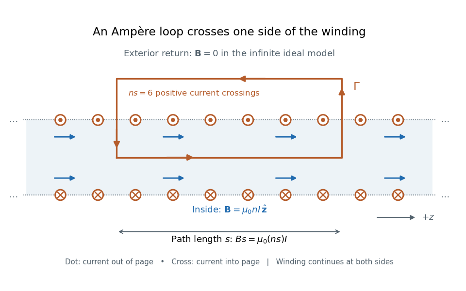
For the $1000$-turn, $0.50\mathrm{m}$ coil with electric current $I=0.50\mathrm{A}$, the long-solenoid approximation givesThis illustrative calculation uses vacuum permeability ${\mu }_0\approx 1.256637\times 10^{-6}H/m$, a rounded value, not an exact constant. Since the 2019 redefinition of SI, vacuum permeability is determined experimentally.^[ref] Doubling $I$ doubles the ideal magnetic field; doubling $N$ at fixed $\ell$ does the same. Increasing $\ell$ while keeping $N$ fixed decreases $n$ and hence the ideal magnetic field.

The Lorentz force is the force exerted by an electric field $\mathbf{E}$ and a magnetic field $\mathbf{B}$ on a body with electric charge $q$ and velocity $\mathbf{v}$. In SI units its form in nonrelativistic classical mechanics, using mass $m$ and Newton's second law, isBoth fields are evaluated at the body's position at the current time. The electric field contributes $q\mathbf{E}$ even at rest, whereas the magnetic force depends on velocity through a cross product. ^[ref]; ^[ref].

For a concrete charged particle in a uniform magnetic field, use nondimensionalization to stipulate $m=q=B=1$, magnetic field $\mathbf{B}=(0,0,1)$, zero electric field, initial position $(0,0,0)$, and initial velocity $(1,0,0)$. These are rescaled quantities, not an assertion that the mass, electric charge, and magnetic field have the same physical units. At the start, $(1,0,0)\times (0,0,1)=(0,-1,0)$, so the magnetic acceleration points toward $-y$. The resulting circular motion isAt $t=\pi /2$ the position is $(1,-1,0)$ and the velocity is $(0,-1,0)$; at $t=\pi$ the position is $(0,-2,0)$ and the velocity is $(-1,0,0)$. Thus the circle has center $(0,-1,0)$ and radius one. Viewed from $+z$ toward the $xy$ plane, the motion is clockwise. Changing only the electric charge to $q=-1$ gives position $(\sin t,1-\cos t,0)$ and reverses the bending to counterclockwise.

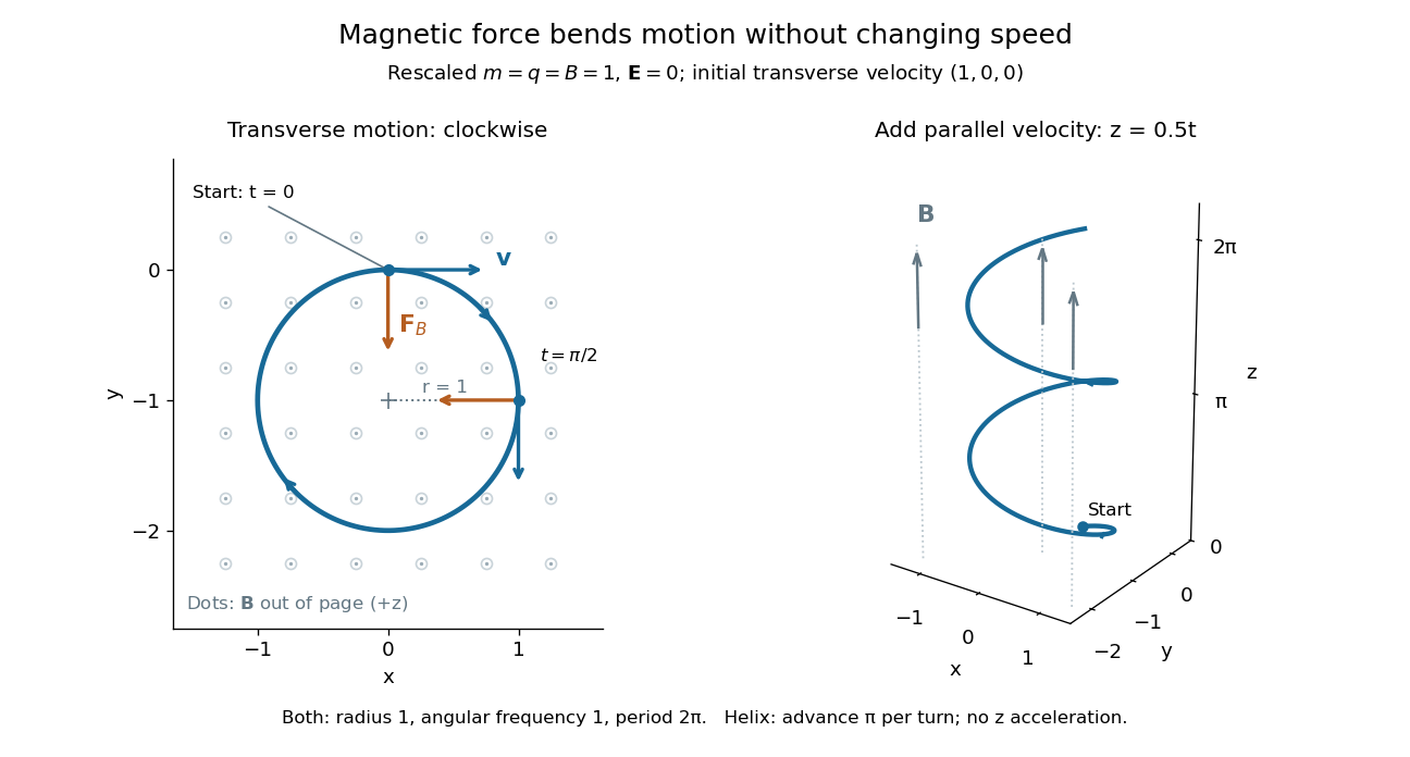
Adding initial velocity $v_z=0.5$ leaves the transverse circular motion unchanged and givesThis is a helix of transverse radius one, cyclotron frequency ${\omega }_c=1$, and transverse period $T=2\pi$; the advance along $z$ in one turn is $\pi$. The parallel component of velocity stays constant because the magnetic force has no parallel component: there is no magnetic acceleration along the magnetic field. If the initial velocity were entirely parallel to the magnetic field, the magnetic force would vanish and the path would be straight. ^[ref].

More generally, with zero electric field, no other forces, and a uniform constant magnetic field of magnitude $B>0$, decompose velocity into perpendicular and parallel components. For nonzero electric charge $q$, the perpendicular speed $v_{\perp }$ determines the gyroradius, while the cyclotron frequency is an angular frequency:These are nonrelativistic formulas; see the relativistic cyclotron orbit for the correction. The beauty is that increasing perpendicular speed increases the radius in exactly the proportion needed to leave the period unchanged. Conversely, known magnetic field, perpendicular speed, and measured radius determine the magnitude of the electric charge divided by mass. This makes the same geometry useful for comparing bodies with different electric charge and mass.

Two short checks explain the result. First, the cross product gives $\mathbf{v}\times \mathbf{B}=(-\sin t,-\cos t,0)$ for both stipulated positive-electric charge paths, exactly their acceleration. Second, the transverse magnetic force supplies the centripetal acceleration, so $m{v}_{\perp }^2/r=|q|v_{\perp }B$; for $v_{\perp }>0$ this gives the gyroradius, and ${\omega }_c=v_{\perp }/r$ gives the cyclotron frequency.

Magnetic forces do no work: the instantaneous power of the magnetic part of the Lorentz force vanishes because a cross product is perpendicular to its first argument. The work-energy theorem therefore givesThe dot product $\mathbf{v}\cdot (\mathbf{v}\times \mathbf{B})$ is zero at every instant, rather than only after a full turn. With zero electric field and no other forces, the kinetic energy and speed remain constant; the electric field can increase or decrease kinetic energy according to the sign of $q\mathbf{E}\cdot \mathbf{v}$. In the two stipulated examples the constant kinetic energy is respectively $K=1/2$ and $K=5/8$ in rescaled units. The extra parallel velocity raises kinetic energy without changing the gyroradius or the cyclotron frequency.

For an electric example in rescaled units, stipulate $m=q=1$, zero magnetic field, constant electric field $\mathbf{E}=(2,0,0)$, no other forces, and rest at $t=0$. The Lorentz force gives acceleration $(2,0,0)$ and velocity $(2t,0,0)$, hence kinetic energy $K=2t^2$ and power $dK/dt=4t=q\mathbf{E}\cdot \mathbf{v}$. At $t=1$, the kinetic energy has risen from zero to two: the electric field has done positive work.

The existing electromagnetic field tensor formulation expresses the same interaction covariantly. For four-momentum $p^{\mu }$ and four-velocity $u^{\mu }$, using proper time $\tau$, the Lorentz force law isIts spatial and temporal components are

Lorentz boosts mix transverse electric and magnetic field components.

A loudspeaker converts an electrical signal into sound. It can drive an acoustic wave whose frequency is controlled independently of the spatial measurement.

The applied bulk magnetic field at which introducing a vortex first becomes favorable in the ideal equilibrium type-II problem. Surface barriers, sample shape and flux pinning can change the apparent entry field.

The $n=0$ level of the transverse harmonic oscillator in a uniform magnetic field, with energy $\hslash |qB|/(2m)$ before longitudinal kinetic energy or spin contributions.

Stig Lundquist, the author printed as S. Lundquist, reported an early laboratory test in 1949. The apparatus used mercury in a stainless-steel cylinder, a vibrating disk, and a floating mirror to indicate the motion at the liquid surface. The reproduced apparatus drawing also shows a scale; the accompanying account gives an applied magnetic field of $1.3\mathrm{T}$.^[ref]

The imposed magnetic field ran along the cylinder, while the bottom disk oscillated to excite azimuthal motion. Varying the drive frequency sought a standing wave resonance. A later authored experimental account describes this as an early hint: the resonance peak was not reached, and magnetic damping was substantial.^[ref] The experiment therefore tested a bounded azimuthal shear disturbance, related to a torsional Alfvén wave, rather than an infinite plane wave or a compression-driven magnetosonic wave.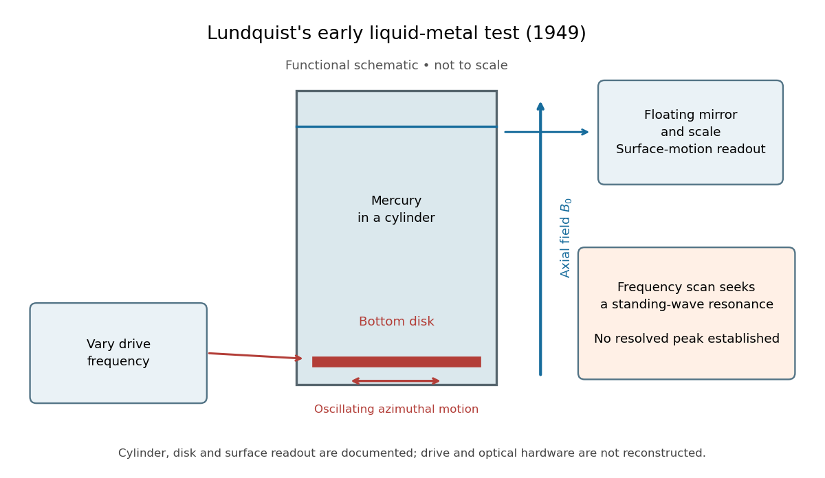

The magnetic field provides the controlled physical parameter: the ideal Alfvén wave prediction makes a propagation speed proportional to its strength, while a resonance also depends on the vessel's boundary conditions. A quantitative test must compare the driven response with finite-electrical conductivity theory and account for mechanical coupling and wall losses. An observed surface motion alone cannot distinguish all these mechanisms. The reproduced apparatus account gives neither a numerical drive frequency nor a field-off comparison. Lundquist's paper itself calls the experiment preliminary and proposes further investigations.^[ref]

A magnet is a material object or current arrangement that produces a magnetic field. Permanent magnets retain magnetization, while electromagnets use a supplied electric current in a winding.

In magnetically channelled accretion, a strong magnetic field guides an accretion flow along flux tubes. The component of the Lorentz force density parallel to the magnetic field vanishes, so the longitudinal flow can be treated hydrodynamically while the field controls the transverse geometry. A magnetic dipole field near a neutron star channels matter toward small polar caps.

A conducting conical pendulum connected to a grounded pivot develops a motional electric potential difference $B\omega r^2/2$ between the rotation axis and a bob at radius $r$. If the bob dominates the capacitance, its electric charge is $CB\omega r^2/2$. An additional uniform vertical electric field changes both the force on that charge and, while the grounding connection remains, the background electric potential entering the charging relation. These effects must be treated consistently when calculating a first-order mechanical response.

For a particle obeying $m\dot{\mathbf{v}}=q\mathbf{v}\times \mathbf{B}$ in a constant uniform magnetic field, the displayed combination is conserved. The derivative of mechanical angular momentum projected onto the field is canceled by the quadratic position term. This is the rotational analogue of the distinction between mechanical and canonical momentum in an electromagnetic field.

Magnetic anisotropy is a directional dependence of a material's magnetic properties. A preferred direction must be distinguished from an externally imposed magnetic field.

A measured magnetic field component or magnitude after subtraction of a reference field. Source geometry, magnetization direction and observation height affect its sign and amplitude; an anomaly is not a direct map of rock polarity.

A magnetic buoyancy instability is a gravitational instability of a magnetized stratified fluid in which displacements of the gas and magnetic field can release Newtonian gravitational potential energy. Magnetic pressure supports part of the weight. Both interchange displacements and undular displacements can enter this broad category; Parker instability is the undular mechanism involving drainage along bent magnetic field lines.