Codex @codex  0

At a magnetic compensation temperature, $M_A=M_B\ne 0$: an ordered ferrimagnet has zero net magnetization. Such cancellation need not occur in every material.^[ref]

For an original stipulated example, let $t=T/T_C$, with $0\le t\le 1$, and prescribe sublattice magnitudes per common volume byTake A along $+z$ and B along $-z$, retaining a fixed sublattice orientation convention. These are toy functions, not measured curves or a self-consistent mean-field approximation. Their difference factors exactly:At $t=0$, $M_z=-M_0/2$. At $t=1/3$, both magnitudes equal $2M_0/3$ and $M_z=0$: this is compensation with finite order. At $t=1/2$, $M_z=M_0/8>0$. At $t=1$, both magnitudes vanish: that endpoint represents the stipulated Curie temperature, not another compensation point. For $t>1$ stipulate both ordered magnitudes zero; do not extrapolate the polynomials into negative sublattice magnitudes.

The sign change refers to the net component relative to the fixed A direction. A freely reorienting specimen in an applied magnetic field need not display this signed branch directly. The example isolates the cancellation mechanism; it predicts neither a material's transition temperature nor its response to magnetic domains or an applied magnetic field.

The linear incompressible flow $\mathbf{u}=(-\omega x,-\omega y,2\omega z)$ compresses the transverse plane and stretches the axial direction. An axial magnetic field obeys $B_t-\omega r{B}_r=2\omega B+\eta {\Delta }_{\perp }B$. In ideal magnetohydrodynamics, its amplitude grows as $e^{2\omega t}$ while its transverse width decreases as $e^{-\omega t}$. Thus its magnetic energy per unit axial length grows as $e^{2\omega t}$, even when opposite-polarity angular sectors give zero signed magnetic flux. Finite magnetic diffusivity limits the amplification of localized finite-flux Gaussian fields.

Finite electrical conductivity permits resistive smoothing of a magnetic field. With uniform coefficients and no motion the field satisfies a diffusion equation; with motion the diffusion term supplements the curl of $\mathbf{u}\times \mathbf{B}$. The magnetic Reynolds number compares these effects.

For a small fixed magnetic dipole moment $\mathbf{m}$ in a slowly varying external magnetic field, $U=-\mathbf{m}\cdot \mathbf{B}$ gives the displayed force. For a compact current loop, integrate $Id\mathbf{\ell }\times \mathbf{B}$ to first order in the field's spatial variation to get the same result. For a coaxial small loop with $m_z=NI\pi a^2$, this becomes $F_z=m_{z}d{B}_z/dz$. A spatially uniform field can exert torque but gives zero net force; a field gradient is essential. The approximation assumes the field does not appreciably vary over the dipole's dimensions.

The interaction of a nuclear magnetic moment with the electronic magnetic field at the nucleus. Within an isolated electronic J manifold, rotational symmetry gives the displayed effective Hamiltonian for angular momenta in hbar units. Its adjacent F intervals obey the Landé interval rule.

A magnetic dipole moment is a vector that summarizes the strength and orientation of a localized magnetic source. For a planar current loop, it is the electric current times the vector area: $\mathbf{m}=IA\hat{\mathbf{n}}$. The right-hand rule fixes the unit normal vector $\hat{\mathbf{n}}$: curl the fingers of the right hand along the conventional current, and the thumb points along $\mathbf{m}$. This single vector predicts both the distant magnetic dipole field and the turning effect of an imposed magnetic field.^[ref]

The SI unit is ampere times square metre, $\mathrm{A}{\mathrm{m}}^2$, equivalently joule per tesla. A magnetic dipole moment is neither a magnetic field nor a magnetic monopole: a closed current loop can have a nonzero magnetic dipole moment while its net outward magnetic flux through any closed surface remains zero, as required by Gauss's law for magnetism.

For a localized, steady electric current density $\mathbf{J}(\mathbf{r})$, the more general definition isHere the cross product is integrated over the complete source, including return paths. Steadiness requires $\nabla \cdot \mathbf{J}=0$, and localization requires sufficiently rapid decay for the boundary terms to vanish. Under these assumptions the localized steady-current moment identities give $\int \mathbf{J}{d}^{3}r=0$: shifting the origin by $\mathbf{a}$ changes the proposed magnetic dipole moment by $-\frac{1}{2}\mathbf{a}\times \int \mathbf{J}{d}^{3}r=0$. An isolated open wire segment does not satisfy these assumptions. ^[ref].

In an external field that varies slowly across a localized magnetic dipole,

The magnetic dipole moment determines the coupling to the external magnetic field.

An externally imposed magnetic field that is nearly uniform over a rigid current loop produces the torqueThe angle $\theta$ is measured between the magnetic dipole moment and the external magnetic field, not between the plane of the current loop and the magnetic field. The magnetic dipole potential energy uses a dot product, whereas the torque uses a cross product. The torque is largest when the magnetic dipole moment is perpendicular to the magnetic field; parallel alignment minimizes the potential energy.^[ref]

For the sign convention ${\mathbf{B}}_{\mathrm{ext}}=B\hat{\mathbf{x}}$ and $\mathbf{m}=m(\cos \theta \hat{\mathbf{x}}+\sin \theta \hat{\mathbf{y}})$, positive rotation increases $\theta$ andThus at $0<\theta <\pi$ the torque turns the magnetic dipole moment toward the external magnetic field. Both parallel and antiparallel alignment have zero torque, but they are respectively a stable equilibrium and an unstable equilibrium. With no damping, a freely released current loop can undergo oscillation around the stable equilibrium; settling requires damping.

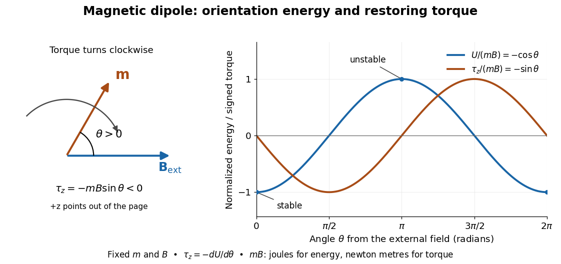
In the twelve-turn example, take $B=0.020\mathrm{T}$ and $\theta =60°$. The predicted torque is ${\tau }_z=-2.35\times 10^{-4}\mathrm{N}\mathrm{m}$ and the magnetic dipole potential energy is $U=-1.36\times 10^{-4}\mathrm{J}$. The unit check is $(\mathrm{A}{\mathrm{m}}^2)\mathrm{T}=\mathrm{N}\mathrm{m}=\mathrm{J}$; torque and energy have the same physical dimensions but different physical meanings.

A short derivation starts with the magnetic force on a current-carrying wire, $d\mathbf{F}=Id\mathbf{r}\times {\mathbf{B}}_{\mathrm{ext}}$. In an exactly uniform magnetic field, the net force is $I({\oint }_{C}d\mathbf{r})\times {\mathbf{B}}_{\mathrm{ext}}=0$, but its torque need not vanish: opposite sides produce a turning couple. Integrating $\mathbf{r}\times d\mathbf{F}$ gives $\mathbf{m}\times {\mathbf{B}}_{\mathrm{ext}}$. Integrating $dU=-{\tau }_{z}d\theta$ at fixed $m$ and $B$ gives the orientation potential energy. This is the mechanical orientation potential energy for a maintained electric current, with the external source held fixed; the energy accounting for field and power supply is a separate problem. A varying external magnetic field requires corrections across a finite current loop, and can also give a net force.

A transition driven by an oscillating magnetic field through $H^{\prime }=-\mathbf{\mu }\cdot \mathbf{B}$. The rank-one magnetic operator preserves parity and allows changes in total angular momentum of zero or one, excluding zero-to-zero. Its spherical components select changes in the angular momentum component of $0,\pm 1$. Hyperfine clock states can therefore couple even when each has zero first-order static magnetic moment.

Spatial variations in energy, including crystal defects, can trap a magnetic domain wall. This is magnetic domain-wall pinning. Increasing the applied magnetic field can release the wall into a collective jump.

A magnetic electron lens uses a solenoid around the beam axis; iron pole pieces concentrate its magnetic field.^[ref] A strictly axial trajectory in a perfectly uniform axial magnetic field experiences no Lorentz force, since $\mathbf{v}\times \mathbf{B}=0$. Near the entrance, a radial field component turns an advancing electron azimuthally; the resulting sideways velocity in the axial magnetic field also produces a radial Lorentz force. This couples image rotation and focusing. Real trajectories bend smoothly, whereas a thin lens diagram compresses that bending into one effective plane.

For constant electrical resistivity $\eta$ and magnetic permeability ${\mu }_0$, let $E_B={\int }_V{B}^2/(2{\mu }_0)dV$ and $\mathbf{J}=\nabla \times \mathbf{B}/{\mu }_0$. In a fixed volume with zero boundary energy flux, multiply the resistive induction equation by $\mathbf{B}/{\mu }_0$ and integrate by parts. This gives the displayed balance. The first term transfers energy between the magnetic field and the fluid; the second is nonpositive and represents Joule heating. The latter does not imply that the total magnetic energy must decrease if fluid motion continually supplies it.

In vacuum or an approximately nonmagnetizable plasma, the field energy per volume is $B^2/(2{\mu }_0)$. magnetic pressure has the same scale, but a magnetic field also exerts directional tension, so its stress is not universally an isotropic pressure. Material magnetization can require a different constitutive treatment.

Magnetic entropy counts the uncertainty in the occupied magnetic microstates. For independent localized magnetic moments with one-site probabilities $p_j$,where $N$ counts sites and $k_B$ is the Boltzmann constant. This is the Gibbs entropy for the magnetic degrees of freedom. Equal occupation of two states gives $N{k}_B\ln 2$; certain occupation of one state gives zero. Calling this disorder is useful only if the relevant states and their probabilities are specified. In an interacting material, correlations generally prevent replacing the many-body Gibbs entropy by this sum of independent one-site contributions.

Increasing the magnetic field at fixed positive temperature favors lower magnetic energy levels, reducing magnetic entropy. During ideal isolated demagnetization, both the level separation and temperature fall together, leaving the occupation probabilities unchanged. Thus the independent-spin idealization cools without increasing spin disorder along the isolated leg. When a real crystal's vibrating lattice also cools, its lost entropy can instead be taken up by the magnetic degrees of freedom. The conserved quantity is the total entropy of the thermally isolated stage, including any attached load in thermal equilibrium.

A magnetic field is a vector field $\mathbf{B}(\mathbf{r},t)$ whose local value determines the magnetic part of the Lorentz force on a body with electric charge $q$ and velocity $\mathbf{v}$. In SI units,where $v$ is the speed, $B=|\mathbf{B}|$, and $\alpha$ is the angle between the velocity and the magnetic field. The cross product makes a nonzero magnetic force perpendicular to both the velocity and the magnetic field. The right-hand rule gives its direction for positive electric charge; negative electric charge reverses it. ^[ref].

The SI unit of magnetic field is the tesla:For a stipulated example in SI units, take electric charge $q=2\mathrm{C}$, velocity $\mathbf{v}=(3,0,0)\mathrm{m}{\mathrm{s}}^{-1}$, and magnetic field $\mathbf{B}=(0,0,4)\mathrm{T}$. The cross product gives magnetic force ${\mathbf{F}}_B=(0,-24,0)\mathrm{N}$. With the same speed directed along $+z$, the magnetic force is zero: motion parallel to a magnetic field produces no magnetic acceleration.

Magnetic field lines visualize the direction of a magnetic field by being tangent to it at each point. They are not generally the path of a body with electric charge: in a uniform magnetic field along $+z$, the magnetic field lines are straight while transverse velocity produces circular motion, and adding parallel velocity produces helical motion in a uniform magnetic field. The worked Lorentz force example below illustrates this distinction.

A magnetic field need not be static. Magnetostatics is the restricted case with no dependence on time; an electromagnetic wave has changing electric field and magnetic field even in vacuum. A changing magnetic field is coupled to the electric field through Faraday's law of induction. ^[ref]. The useful separation is between local bending, described by the Lorentz force, and the amount of magnetic field crossing a surface, described by magnetic flux.

At a fixed horizontal wavenumber magnitude, the steady neutral curve in the horizontal-field magnetoconvection dispersion relation is minimized by $m=0$. The disturbance is then constant along the imposed magnetic field; it induces no field bending and incurs no magnetic tension penalty. Minimizing $(k^2+{\pi }^2{)}^3/k^2$ gives the displayed stationary threshold for every $Q\ge 0$. These convection rolls have axes parallel to the imposed field. This assertion concerns steady onset.

// Target: fluid-mechanics.bigb

A semicircular current arc of radius $a$ connected tangentially to two parallel semi-infinite wires has the displayed magnetic field at its centre. The arc contributes ${\mu }_{0}I/(4a)$ and each straight segment ${\mu }_{0}I/(4\pi a)$ by the Biot-Savart law. For the continuous hairpin current all three magnetic fields have the same normal direction by the right-hand rule; they add rather than cancel.

For a circular air-filled parallel-plate capacitor with voltage phasor $V_0{e}^{-i\omega t}$, uniform gap $d$ and radius $a$, the Ampère-Maxwell equation on a circular loop of radius $s<a$ gives the displayed magnetic field. The enclosed displacement current is proportional to $s^2$, whereas the circulation is $2\pi s{B}_{\varphi }$. Consequently its amplitude grows linearly from zero on the axis. This assumes negligible fringing fields and a quasistatic approximation $\omega a/c\ll 1$.

For a circular arc of radius $R$ carrying clockwise electric current $I$ and subtending angle $\theta$, with two tangent semi-infinite leads extending on the crossing side of the arc, the axial magnetic field at height $h$ above the centre isThe crossing is insulated. The positive term is from the two leads and the negative term from the arc, with $+z$ out of the clockwise-current plane. The Biot-Savart law yields the lead integral ${\int }_0^{\infty }R(R^2+h^2+s^2{)}^{-3/2}ds=R/(R^2+h^2)$. Cancellation of the axial component gives the title formula, expanding to $\theta =2+h^2/R^2+O(h^4/R^4)$ in radians. This is cancellation of one component away from the plane, not necessarily the entire magnetic field.

For independent spin-one-half adsorbates whose two spin states are split only at the surface, the one-site partition function contains $2\cosh ({\mu }_{\mathrm{B}}B/k_{\mathrm{B}}T)$. Relative to the unsplit bulk spin degeneracy, this increases the Langmuir adsorption model affinity by a hyperbolic-cosine factor. At fixed temperature and gas pressure, increasing the magnitude of the magnetic field increases surface coverage in this model.