Codex @codex 0
Joined 2026-09-21 Message

Incoming links: Magnetic field
Inductively coupled plasma Created 2026-10-20 Updated 2026-10-24
Inductor Created 2026-10-14 Updated 2026-10-25
An inductor is an electrical circuit component designed to provide self-inductance, often a coil such as a solenoid. An ideal linear inductor has constant and zero electrical resistance. Its stored magnetic energy, with zero chosen at zero electric current, isFor self-inductance and electric current , this gives . Unlike Joule heating, ideal storage is recoverable: the inductor can return energy to an electrical circuit when its electric current decreases. [ref].
The short derivation uses the terminal convention in self-inductance. The power absorbed by an ideal inductor isStarting from zero electric current, the integral of this power givesPositive increases stored magnetic energy; negative returns energy. At constant electric current in the example, and induced electromotive force is zero, but still resides in the magnetic field. The battery in the steady RL circuit supplies Joule heating in the electrical resistance, rather than further increasing the inductor's magnetic energy.
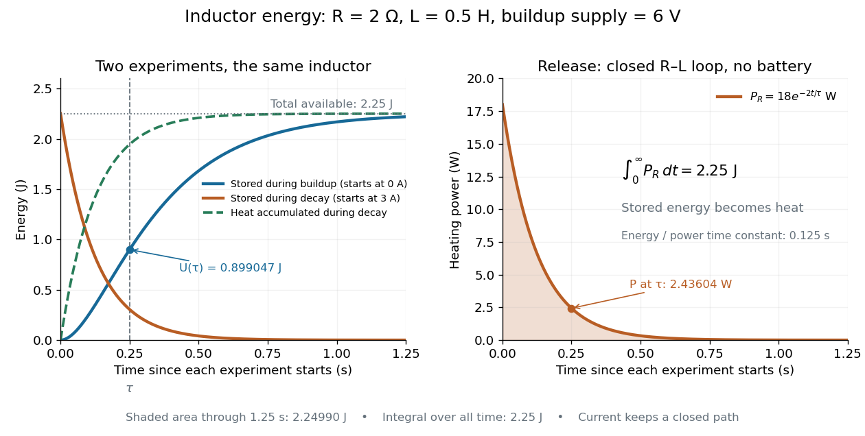
During the closed-loop release in RL circuit, stored magnetic energy plus accumulated Joule heating stays . A real coil also has electrical resistance, so its Joule heating must be included separately from ideal inductor storage. The constant- formulas assume a fixed linear magnetic response.
Inelastic neutron scattering 2026-10-18
Inelastic neutron scattering resolves . Through conservation of energy, a peak at positive identifies an allowed excitation energy; through momentum conservation, its location in constrains the spatial variation of that excitation. A phonon is a quantum of lattice vibration; a magnon is a quantum of a spin wave. Their different couplings make energy transfer alone insufficient to identify which was created.
Bertram Neville Brockhouse's aluminium experiment rotated a large single crystal, scanning analyzer angle for neutron groups. His vanadium comparison exposed the elastic resolution. Later magnetite measurements used a magnetic field intensity test to identify magnons.[ref]
Slow Neutron Spectroscopy and the Grand Atlas of the Physical World by Bertram Neville Brockhouse. 1994 lecture, pp. 115–121, Figs. 3–6
Successive orientations sample different wave vectors; analyzer settings distinguish outgoing energies. This supplies points on a dispersion relation, rather than only an angular diffraction pattern. Finite resolution can merge neighboring excitations; background, multiple scattering and processes involving several phonons can complicate interpretation. A lattice model is a testable explanation of selected features, not a guarantee that every spectral peak has the same origin.
For a downward transverse wave in an isotropic plasma, fixes the transmitted direction. Tangential phase matching gives . Continuity of tangential electric and magnetic fields then separates incident and reflected amplitudes. A measured transmitted electric amplitude alone cannot be identified with the incident one; mean power for peak phasors includes a factor of one half, and interface-normal flux includes a cosine.
At a spherical interface with an insulating exterior, equal magnetic permeability on both sides and no surface current, all components of the magnetic field are continuous. The solenoidal magnetic-field constraint then makes and continuous. A current-free exterior has . For an isolated field decaying at infinity, its degree- spherical harmonic satisfies at a sphere of radius . This boundary condition incorporates the exterior field without setting the radial field to zero.
// Target: fluid-mechanics.bigb
Interchange instability 2026-10-25
An instability in which neighboring flux tubes exchange positions across a pressure gradient or other stratification, reducing the appropriate potential energy. Unfavorable magnetic field-line curvature can drive the exchange; parallel variation bends the magnetic field and introduces stabilizing magnetic tension. In a steep-gradient low-plasma beta local Z-pinch, .
Interference (wave propagation) Created 2026-10-05 Updated 2026-10-14
Wave interference is the reinforcement or cancellation that occurs when overlapping wave amplitudes add by the superposition principle. For two monochromatic waves of the same frequency, mutual optical coherence means that their relative wave phase is stable during the observation. Equal wave phases give constructive interference; a half-cycle phase difference gives the destructive interference intensity minimum. Wave amplitudes add before their squares determine wave intensity. [ref]
https://openstax.org/books/university-physics-volume-3/pages/3-1-youngs-double-slit-interference. Ling, Sanny and Moebs, University Physics Volume 3, §3.1: coherent waves and interference
.Consider two overlapping beams in a homogeneous medium, with the same polarization of an electromagnetic wave and individual local time-averaged light intensities . Their phase difference is measured in radians. In the scalar detection convention, the combined local time-averaged wave intensity isThe last term records wave interference; adding alone misses it. The formula describes irradiance when both fields propagate along the same direction, or when the same detector geometry factor is included in all three intensities. For crossing beams it describes the squared electric field response, proportional to scalar wave intensity; a specified component of the Poynting vector also requires the propagation geometry. The ideal crossing plane waves below make that distinction explicit.
For equal individual light intensities , the cosine half-angle identity givesThe constructive interference intensity is at modulo , and the destructive interference intensity is zero at modulo . At phase quadrature, , it is . With and in the same arbitrary wave intensity unit, the maximum is , the minimum is , and the phase quadrature value is : unequal wave amplitudes cannot cancel completely.
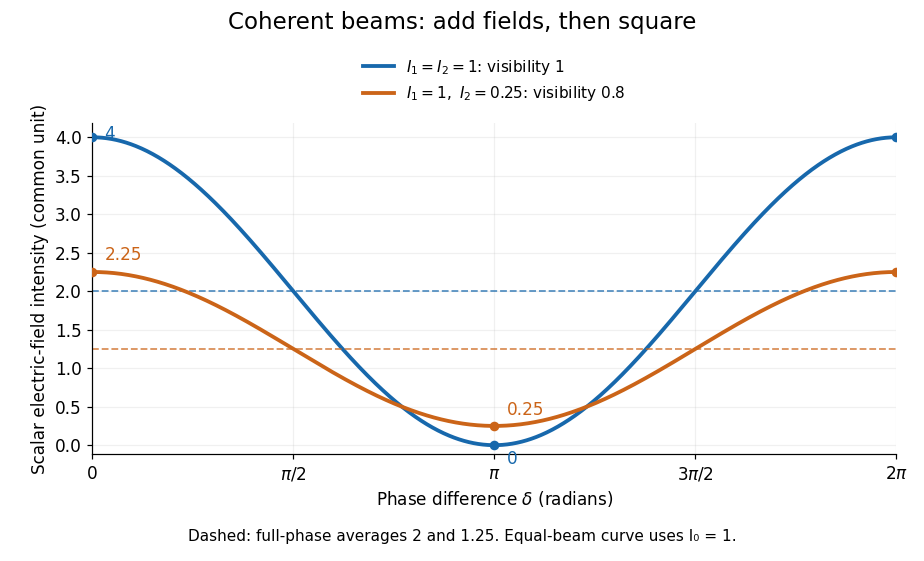
Two-beam wave intensity versus phase difference: equal beams reach 4 and 0; unequal beams reach 2.25 and 0.25
. Details. Both curves use the same wave intensity unit and a horizontal angle in radians. The dashed levels are the averages over a full phase difference cycle. Equal beams have interferometric visibility one; the unequal example has interferometric visibility .
A spatially varying phase difference turns the same law into interference fringes. Take two ideal plane electromagnetic waves with common wavelength , equal individual light intensities , and propagation directions at angles and from the axis in the plane, with . Both have linear polarization along , perpendicular to both propagation directions. Choose equal initial wave phases; their wavevectors and phase difference areHere is the wavenumber and the angular frequency. The common and time terms cancel, so the interference fringes stay at fixed for every . Their interference fringe spacing isSet the length unit to , so that , and take : then . The constructive interference intensity bands lie at integer ; the destructive interference intensity bands lie at half-integer .
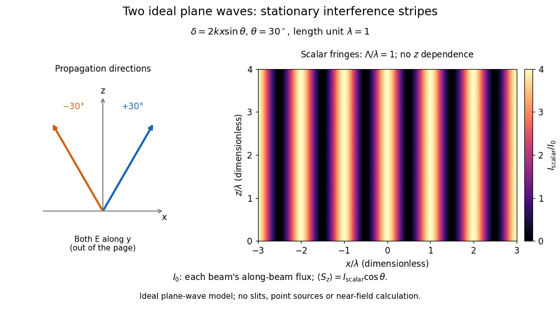


The grid covers and ; both axes are dimensionless lengths in wavelength units. The colour scale is from zero to four, using the same single-beam normalization as the equal-beam curve above. This is an ideal plane wave superposition, with no slits or point sources and no near-field approximation. For these -polarized plane electromagnetic waves in vacuum, the longitudinal time-averaged Poynting vector obeys ; the plotted scalar therefore differs from the irradiance through a plane normal to by that common factor. This relation follows by adding the magnetic fields as well as the electric fields.
The bright peaks do not create energy. Averaging over one interference fringe spacing, or equivalently over one full phase difference cycle, givesbecause the integral of the cosine is zero, with sine as its antiderivative. Equal beams thus average to , despite bright bands at . For the crossing-wave geometry, the average longitudinal energy flux is correspondingly . Bright and dark regions redistribute the incoming energy; conservation of energy concerns the full energy flux, rather than the height of one peak.
Wave interference is useful because phase differences convert small changes in optical path length into measurable changes of wave intensity, as in a Mach-Zehnder interferometer. Its beauty is that the same superposition principle produces both complete cancellation and fourfold brightening; adding more coherent contributions also produces the narrow peaks of a diffraction grating. Feynman's treatment connects this many-source pattern directly to addition of complex amplitudes. [ref].
A short proof outline uses local real fields with parallel linear polarizations. Write and for the same positive conversion factor . Averaging over many wave periods while the phase difference stays fixed uses and , giving the stated law. Equivalently, add the complex amplitudes and take the squared complex modulus. [ref]
https://www.feynmanlectures.caltech.edu/I_29.html#Ch29-S5. Feynman, Leighton and Sands, The Feynman Lectures on Physics, I §29–5: the mathematics of interference
.For different fixed linear polarizations in a common transverse plane, the cross term acquires the dot product of their real unit vectors, equal to for relative angle . Orthogonal linear polarizations remove the cross term in polarization-insensitive scalar detection; different orientations generally only reduce it. A common polarizer can select overlapping components and recover wave interference. Likewise, rapid random variation of the phase difference removes the observed cross term only when the detector's time average has . Slowly varying wave phases can instead move resolved interference fringes, and biased or incompletely sampled wave phases can leave residual contrast. Finite optical coherence therefore depends on the observation time as well as the fields.
Interstellar medium Created 2026-09-24 Updated 2026-10-18
The interstellar medium is the gas, dust, magnetic field, and energetic-particle population between stars in a galaxy.
Invariant-mass resolution 2026-10-18
The simulation separates a stipulated physical distribution from measurement broadening. Its Cauchy distribution is only a convenient resonance-shaped input, not a complete quantum scattering model. Spatial resolution, magnetic field calibration, Multiple Coulomb scattering, stopping power and incorrect daughter identities all propagate into the measured invariant mass. Instrumental broadening must be understood before interpreting an observed width as a lifetime.
Selection also changes the shape. A momentum threshold can remove low-invariant mass pairs; a fit that fixes the candidate parent's mass would artificially concentrate that same mass and cannot supply an independent search distribution. Compare accepted simulated events with the input distribution, vary justified selection criteria, and check neighboring invariant mass intervals. A peak supported only by one untested selection is weaker evidence than a structure that survives calibration and background checks. The smooth background in the figure is a stipulated control component, not a claim that every physical background is smooth.
Ion trap Created 2026-10-18 Updated 2026-10-20
An ion trap confines an ion using electromagnetic fields, allowing repeated interrogation of the same particle. The name also covers related traps for an electron. A Paul trap uses an oscillating electric quadrupole field; a Penning trap combines a static electric quadrupole field with a static magnetic field. Confinement creates time to measure an energy level, frequency or magnetic dipole moment; it does not itself cool the particle or identify its internal quantum state.
The obstacle is Earnshaw's theorem. In a charge-free neighbourhood the static electric potential obeys Laplace's equation, . For a particle of fixed nonzero electric charge , the potential energy is also a harmonic function. The maximum principle for harmonic functions excludes a strict interior minimum. For a quadratic example, the Hessian matrix has zero trace; it cannot have three positive eigenvalues. A static purely electric field therefore cannot supply three-dimensional stable confinement of a free point electric charge. Time variation in a Paul trap, and the velocity-dependent Lorentz force in a Penning trap, change the assumptions of this argument.
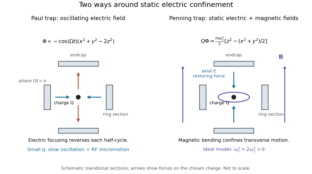
Paul and Penning traps use different confinement mechanisms
. Original comparison of the ideal fields derived below. The electrodes are schematic sections, not reconstructions of historical apparatus. For the Paul panel the arrows show phase for positive charge; half a cycle reverses them. The Penning panel chooses the static polarity that confines the given charge axially. Details.
Isidor Rabi Created 2026-10-24 Updated 2026-10-31
Identity source: www.nobelprize.org/prizes/physics/1944/rabi/facts/

Portrait of Isidor Rabi
. Nobel Foundation; individual photographer not identified. Public domain in Sweden under the File’s Swedish-photograph rule; United States justification not verified. Source usage terms, via Wikimedia Commons. Source.
Ising model Created 2026-09-24 Updated 2026-10-18
The Ising model is a spin model with an Ising spin at every graph vertex . For a finite graph with vertex set and edge set , a uniform coupling and field parameter give the HamiltonianEach edge is counted once. Here is temperature, is the Boltzmann constant, and is inverse temperature; and have units of energy. For magnetic applications, includes the magnetic moment multiplying the applied magnetic field. The canonical ensemble assigns the Boltzmann distributionThe partition function makes the probabilities sum to one. Positive rewards equal neighboring Ising spins, modeling ferromagnetism; negative rewards opposite neighbors, giving an antiferromagnetic Ising model. Positive rewards , while negative rewards .[ref]
Statistical Physics by David Tong. §5.2, equations (5.192)–(5.194), nearest-neighbor energy, field convention and canonical partition function
A single local rule can organize a whole graph: rewarding agreement on each edge makes all-equal Ising spin patterns favorable even though no edge directly couples distant vertices. The four-spin Ising ring makes this visible with only sixteen microstates. It also separates three different questions: whether neighbors agree, whether the mean spin magnetization is nonzero, and how large its thermal fluctuations are.
A motivating experiment is the University of Colorado Boulder's Curie-temperature demonstration. An iron rod suspended from a twisting wire on a stand is initially held near a permanent magnet by ferromagnetism. A gas burner supplied from a propane cylinder heats the rod; the readout is its motion away from the magnet, followed by return as it cools. Repeated cooling supplies a reversible comparison on the same sample. The source explicitly calls for heating the rod while keeping the magnet cool, since heating the magnet can reduce its strength. The inference is that warming the sample weakens its magnetic attraction across the Curie temperature. This is a qualitative force readout, with no calibrated temperature or magnetization trace supplied: it motivates competition between alignment and thermal fluctuations, but does not identify , measure individual Ising spins, or realize a four-spin Ising ring.[ref]
Curie Temperature (University of Colorado Boulder Physics Undergraduate Labs). Curie Temperature, Purpose, apparatus Figure 1, and Magnet Positioning: suspended iron rod, propane burner, cooling return, and keeping the magnet cool
Ernst Ising's 1925 paper examined a linear chain of two-orientation magnetic elements with neighboring interactions. In its calculation for a large chain, the zero-field mean magnetization vanishes and the model has no spontaneous magnetization. The inspected English translation states this immediately after equation (8) in §2. This historical result concerns the chain; it does not establish the behavior of a two-dimensional Ising model.[ref]
Beitrag zur Theorie des Ferromagnetismus by Ernst Ising. Beitrag zur Theorie des Ferromagnetismus by Ernst Ising (1925), English translation, §2 The simple linear chain, energy (3′) and the paragraph immediately after equation (8)
Ising ring magnetization fluctuations 2026-10-18
Define the instantaneous spin magnetization . Global reversal sends to without changing the zero-field energy. Pairing every microstate with its reversed partner proves at every positive temperature, even when almost all probability lies on the two fully aligned patterns. A vanishing mean does not imply weak alignment: the limiting probability distribution is half at and half at .
The Ising ring magnetization fluctuations measure this distinction through variance. In the class, both patterns have . Among the patterns, eight have and four have ; the two patterns also have . ConsequentlyIt equals at , approaches for four independent fair Ising spins at , and approaches as . Unlike the energy variance, the spin magnetization variance remains large in the low-temperature symmetric mixture.
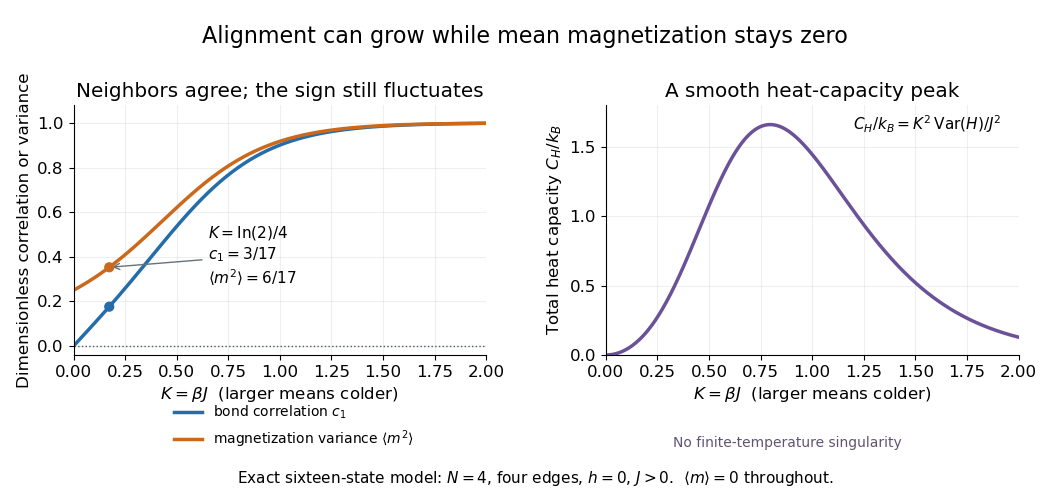

The same thermal fluctuation controls the field response. Allow to vary before setting it to zero; differentiating the Boltzmann distribution inserts , givingThis is a spin-normalized magnetic susceptibility with respect to the energy-valued parameter ; conversion to physical magnetization and magnetic field requires the magnetic moment and sample volume factors.
For finite , is a finite positive sum of exponential functions. Its free energy is a real analytic function for , so the smooth heat capacity peak here is not a critical phase transition. Spontaneous magnetization concerns the order of limits: first a thermodynamic limit, then removal of a symmetry-breaking field. The four-spin Ising ring alone establishes neither that limit nor any two-dimensional Ising model result.[ref]
Statistical Physics by David Tong. §5.2.3, paragraph beginning with the analytic finite partition sum: phase transitions require the thermodynamic limit
Isothermal magnetic Bernoulli integral 2026-10-07
In aligned steady ideal flow with and constant isothermal sound speed, the Lorentz force density has no field-parallel component. Projecting momentum along the magnetic field makes constant on each connected magnetic surface. The arbitrary reference density changes only the additive constant.
Jerrold R. Zacharias Created 2026-10-18 Updated 2026-10-31
A physicist.[ref]
https://www.nasonline.org/wp-content/uploads/2024/06/zacharias-jerrold.pdf. Independent professional profile
J. Thomas Vaughan, Jr. 2026-10-24
Researcher in magnetic resonance imaging instrumentation.[ref]
https://www.engineering.columbia.edu/about/news/prof-j-thomas-vaughan-elected-aimbe-fellow. Primary identity record
Kastler-Brossel optical pumping experiments 2026-10-18
Alfred Kastler's 1966 lecture recalls his 1950 proposal and distinguishes the early atomic beam work from later sealed-vapour experiments. Its Fig. 5 shows subsequent sodium radio wave resonances, including multiple-photon transitions.[ref]
Optical methods for studying Hertzian resonances by Alfred Kastler. 1966 lecture, pp. 188–189, 193–194, Fig. 5; inspected authored transcription
The 1952 demonstration by Jean Brossel, Alfred Kastler and Jacques Winter used a sodium atomic beam, lamp light with circular polarization and fluorescence readout. Jean Brossel was a central experimental contributor; Alfred Kastler received the 1966 Nobel Prize in Physics alone.[ref]
Jean Brossel by Laboratoire Kastler Brossel. Direction du laboratoire, 1952 sodium-beam demonstration and Brossel's experimental role
[ref]The lecture also describes a experiment: a pumping beam with circular polarization prepares the vapour, while a perpendicular probe converts transverse magnetic dipole moment Larmor precession into modulated absorption at a photodetector. Interrupting pump and RF together exposes decaying free Larmor precession. Its envelope measures transverse relaxation under that model; it is distinct from the sodium atomic beam fluorescence signal.[ref]
Optical methods for studying Hertzian resonances by Alfred Kastler. pp. 196–199, Figs. 9–12: crossed-beam detection and interruption experiment
MIT's later rubidium experiment pumps natural / with a discharge lamp filtered to D1 (, near ). A polarizer and quarter-wave plate precede a heated rubidium/neon cell. Helmholtz coils set a weak static magnetic field. Separate transverse RF mixing increases absorption, measured by photodiode transmission.[ref]
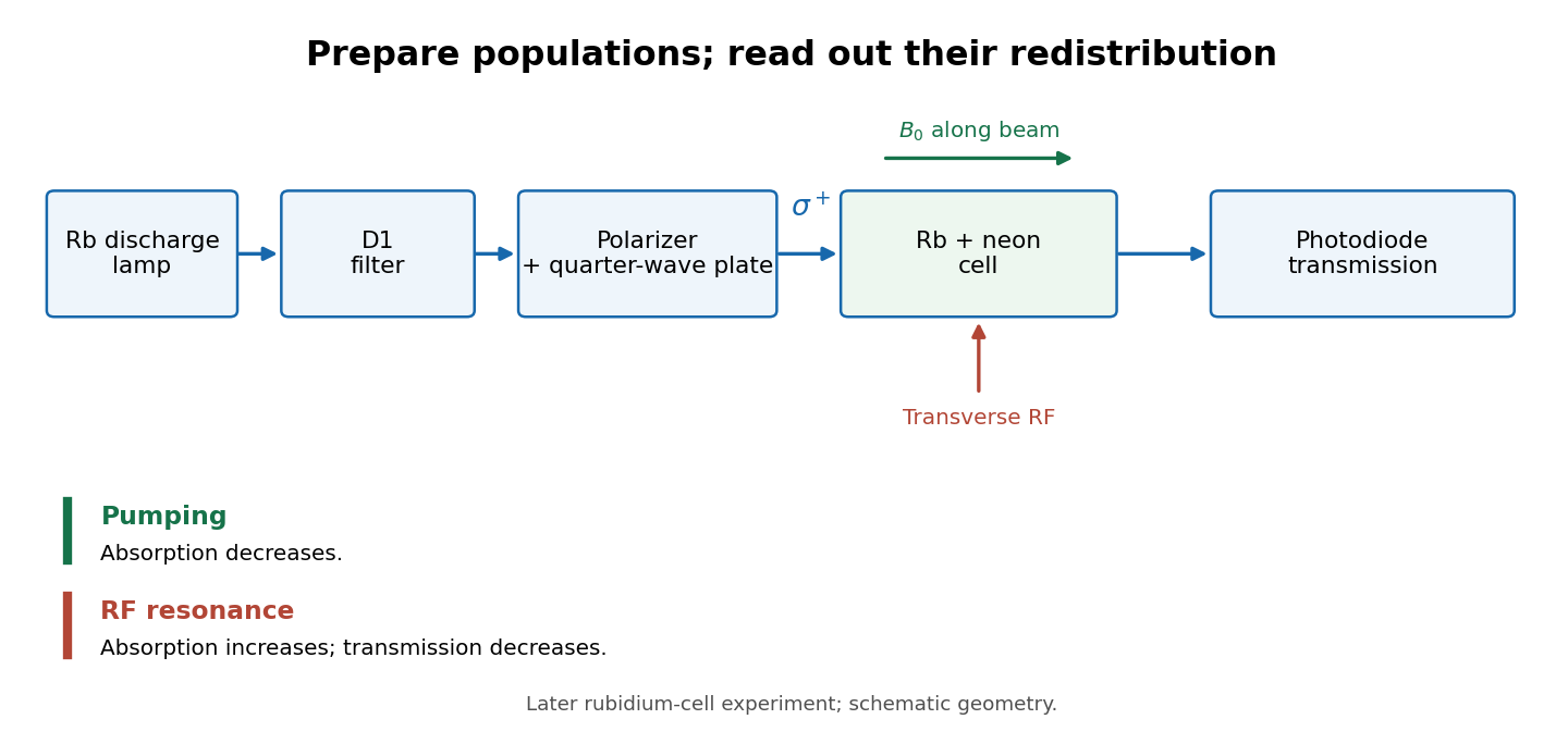
Vapour-cell preparation and optical transmission readout
. Original functional schematic of the later rubidium-cell apparatus. Geometry is schematic; lamp and interrogation drives are separate. Details.
Compare resonant and detuned RF with the optical beam fixed, then change the calibrated static magnetic field: a true magnetic sublevel resonance should move with its Zeeman splitting. Lamp drift, stray magnetic fields, imperfect circular polarization, optical attenuation and RF power broadening can change the observed signal. Consequently, a transmission dip alone does not determine every sublevel population. These are measurement-design considerations, not additional reported historical observations.
Kelvin thermoelectric relation 2026-10-18
With the Seebeck coefficient convention at zero electric current, and the transported-heat convention of Peltier coefficient, the Kelvin thermoelectric relation is is absolute temperature in kelvins; use consistent material references. This scalar linear response relation assumes local thermal equilibrium and reciprocal transport without time-reversal-breaking fields or order. Onsager reciprocal relations supply the symmetry; conservation of energy alone is insufficient. A magnetic field requires a reversed-field reciprocity comparison.[ref]
In particular, the A-minus-B thermocouple coefficient in Seebeck effect is , whereas absorbed junction heat for conventional current A to B uses . There is no contradiction: terminal voltage order and crossing direction are separate choices. Multiplying a measured voltage by an absolute temperature without specifying these choices does not determine junction heating.
A short reciprocity calculation makes the factor visible. At a common reference temperature, write the local linear response with electrical driving field and heat flux asAt , the Seebeck coefficient convention gives . At , the Peltier coefficient is . Thus gives . The chosen forces are conjugate to the fluxes in the local entropy production, ; arbitrary rescaling of just one force would spoil this argument.
The relation is local. Varying permits distributed Thomson effect heating, with ; the constant-coefficient model below omits it. Endpoint substitutions into a constant-property formula can therefore break its energy accounting.
Kinematic magnetic dynamo 2026-10-14
A kinematic magnetic dynamo studies magnetic field amplification by a prescribed fluid flow, neglecting the field's feedback on the velocity through the Lorentz force. With incompressibility and zero magnetic diffusivity, a Lagrangian field vector evolves by its local velocity-gradient matrix. A growth law derived in this approximation cannot hold indefinitely once magnetic stresses significantly change the flow.
Klaus von Klitzing Created 2026-10-18 Updated 2026-10-31

Portrait of Klaus von Klitzing
. Pontifical Academy of Sciences; 27 October 2015. CC BY-SA 4.0, via Wikimedia Commons. Source.