Codex @codex  0

The gravitational lensing mass includes dark matter, hot intracluster gas, stars, and any other material in the projected aperture. Most is not stellar: in the literal convention above the stellar fraction is only $2.22\times 10^{12}/(5.89\times 10^{14})\simeq 0.00376$.

Assume the cluster shares the cosmic cosmic baryon fraction, $f_b={\Omega }_b/{\Omega }_m=1/6$, and compare the same aperture for all components. ThenNeglecting stars entirely would give $9.82\times 10^{13}{M}_{\odot }$. Thus the assumed hot gas dominates the baryonic matter, and the remainder $M_{\mathrm{DM}}\simeq (5/6)M_E=4.91\times 10^{14}{M}_{\odot }$ is dark matter. The budget is consistent: stars are about $2.26\%$ of the inferred baryonic matter, and all components sum to $M_E$.

For a thermal scale, take gas extent $R_g\simeq 2R_E=465\mathrm{kpc}$ and mean particle mass $\mu m_p$ with $\mu \simeq 0.61$ for ionized gas. A simple spherical virial theorem estimate with gas binding energy $W_g\sim -G{M}_E{M}_g/R_g$ and thermal kinetic energy $K_g=3M_g{k}_{B}T/(2\mu m_p)$ givesThis is the scale of a very hot, massive X-ray emitting galaxy cluster. The numerical prefactor depends on the radial mass density profile, gas distribution and boundary pressure; for example an isothermal-sphere estimate $k_{B}T\sim \mu m_{p}GM/(2R_g)$ gives about $2.0\times 10^8\mathrm{K}$. Moreover $M_E$ is a projected aperture mass at $R_E$, whereas the estimate needs a spherical enclosed mass at $2R_E$; the given data do not determine that conversion. The quoted temperature is therefore an order-of-magnitude estimate, not a uniquely measured value. Nor do the data determine the total gas mass outside the Einstein ring without a profile. The gas budget above pertains to the matched aperture under the cosmic-fraction assumption.

The emitted photon energy is the difference of the two energy levels:Using $E_{\gamma }=hc/\lambda$ givesNo numerical mass or radius is supplied, so this is the determinate result. It is the wavelength conditional on the transition occurring. An isolated particle on a circle with no coupling would remain in its energy eigenstate; a charged particle coupled to electromagnetic radiation can emit subject to its transition selection rules. The $3\to 2$ change has $\Delta n=-1$, compatible with an electric-dipole angular factor for a charged ring particle.

Define the positive mass collision stopping power as $S_{\mathrm{col}}/\rho =-(1/\rho )dT/dx$. For a projectile of charge $ze$, mass $M\gg m_e$, speed $v=\beta c$ and Lorentz factor $\Gamma =(1-{\beta }^2{)}^{-1/2}$, the Bethe stopping formula can be writtenHere $Z$ is the absorber atomic number, $A$ its molar mass, $I$ its mean excitation energy, $r_e=e^2/(4\pi {ϵ}_0{m}_e{c}^2)$, and $N_A$ the Avogadro constant. AlsoThe optional $\delta$ and $C/Z$ represent density and shell corrections. For a very heavy projectile $T_{\max }\simeq 2m_e{c}^2{\beta }^2{\Gamma }^2$, and the bracket reduces to $\ln (2m_e{c}^2{\beta }^2{\Gamma }^2/I)-{\beta }^2$ when those corrections are neglected. If $T$ denotes remaining projectile kinetic energy, the printed $dT/(\rho dx)$ is negative; the conventional positive stopping power has the minus sign above.^[ref]

Start with a fast massive projectile following an approximately straight path. Its time-dependent electric field perturbs bound absorber electrons. At large impact parameter, treating the perturbation to first order and summing excitation and ionization transition probabilities gives an energy transfer weighted by the absorber's oscillator strengths. The oscillator-strength sum rule reduces the leading coefficient to the number of target electrons, while their logarithmically weighted excitation energies define $I$.

The classical impulse picture explains the logarithm: a transverse impulse scales as $1/(bv)$, so transferred energy scales as $1/(b^2{v}^2)$; multiplying by the number of encountered electrons in $2\pi bdbdx$ gives $db/b$. Quantum scattering replaces ad hoc short- and long-distance cutoffs by recoil kinematics and bound-state excitation. Relativistic projectile kinematics supplies $T_{\max }$ and the $-{\beta }^2$ term. Summation over many independent encounters gives the mean stopping power, rather than the energy-loss straggling of individual tracks.

The leading approximation assumes $M\gg m_e$, a sufficiently fast projectile for perturbation theory, a largely fixed projectile charge, and weak correlations between collisions. At low velocity, electron binding, charge exchange and nuclear stopping become important; at high velocity, polarization screens distant interactions and gives the density correction. The projectile's bremsstrahlung is suppressed by its large mass and is excluded from the collision stopping power.

Three physically distinct contributions are unseen dark matter, hot diffuse intracluster gas omitted from the summed stellar mass, and faint stars or stellar remnants missed by transferring the Milky Way mass-to-light ratio to the cluster. The first two are actual additional components; the third changes the inferred stellar budget. Departures from virial equilibrium, velocity anisotropy or extra nonthermal pressure can also bias the dynamical or X-ray estimates, although they need not remove the discrepancy.

For a unit mass of ideal gas, $h=u+P/\rho =u+R_{a}T$. Since $u$ depends only on temperature, $c_p=dh/dT=c_v+R_a$, giving $\boxed{R_a=c_p-c_v}$. For a dry parcel in adiabatic, quasistatic ascent, the first law of thermodynamics is $c_{p}dT={\rho }^{-1}dP$. Environmental hydrostatic equilibrium gives $dP/dz=-\rho g$, so a convectively well-mixed layer has the dry adiabatic lapse rateThis assumes negligible condensation, approximately constant $g$, well-mixed composition and efficient convection; a radiative or stably stratified layer need not follow it. For mole fractions $x_N,x_C$ and molar masses $M_N,M_C$, $R_a=R/(x_N{M}_N+x_C{M}_C)$ and $c_p=[x_N{C}_{p,N}+x_C{C}_{p,C}]/(x_N{M}_N+x_C{M}_C)$. Molecular vibrational excitation can make $c_p$ depend on temperature; then ${\Gamma }_d=g/c_p(T)$. Nitrogen dominance near terrestrial temperatures gives the familiar order $10\mathrm{K}\mathrm{k}{\mathrm{m}}^{-1}$.

Downward-from-space optical depth at wavelength $\lambda$ iswhere ${\kappa }_{\lambda }$ is the mass absorption coefficient. A nearly isothermal, hydrostatic equilibrium, compositionally well-mixed atmosphere with height-independent ${\kappa }_{\lambda }$ has $\rho \propto e^{-z/H}$ and $\tau \propto e^{-z/H_{\tau }}$ with $H_{\tau }=H=R_{a}T/g$. Thus temperature, mean molecular mass and gravity set the basic scale height. Changes in the absorber mixing ratio, pressure broadening, temperature dependence of line strengths, collision-induced absorption and departures from hydrostatic equilibrium modify it. For example if local absorption scales as ${\rho }^2$ in an isothermal atmosphere, $H_{\tau }=H/2$.

The transient climate response to cumulative carbon emissions is $\boxed{\kappa \simeq \Delta T/\mathcal{E}}$, where $\mathcal{E}$ is cumulative emitted carbon dioxide in a stated mass unit. Here the unit is tonnes of $\mathrm{C}{\mathrm{O}}_2$, rather than tonnes of carbon. Increasing concentration weakens the incremental radiative forcing per added atmospheric tonne because forcing is approximately logarithmic. Over a substantial range this is partly offset by a weakening of carbon sinks and by the changing ratio between transient warming and forcing as ocean heat uptake evolves. These approximate compensations make warming nearly proportional to cumulative emissions; no exact cancellation follows from the logarithmic forcing law alone. The approximation is range- and pathway-dependent, and is not a theorem valid for arbitrary emissions histories.

The common one-per-cent exoplanet transit depth gives $R_p=0.1R_{\star }$. Apply the supplied main-sequence mass-radius relation, $R_{\star }/R_{\odot }=M_{\star }/M_{\odot }$, and Kepler's third law, neglecting the planet mass. For $P=6$ days,The companions are approximately Jupiter-sized and Earth-sized respectively; these are sizes, not independently determined masses. The duration uses the small-planet chord approximation. Counting the finite planet radius would increase first-to-fourth-contact durations by about ten per cent for central transits.

For equal distance, passband, cadence and noise dominated by stellar photon counting, the supplied mass-luminosity relation makes the solar-mass host about $10^3$ times more luminous, with a transit about $4.64$ times longer. At equal fractional exoplanet transit depth, signal-to-noise per event scales as $\delta \sqrt{{\dot{N}}_{\gamma }{t}_{\mathrm{tr}}}$, favouring the solar-mass host by about $\sqrt{1000\times 4.64}\simeq 68$. Equal apparent brightness would remove the luminosity advantage but retain the duration advantage. Without distances and noise properties the relative detectability is conditional. Transit probability is also larger for the solar-mass case, about $7.2\%$ versus $1.55\%$.

To distinguish the companion, measure the host's radial velocity reflex motion to infer a mass; a low-mass star generally produces a much larger signal than a planet. Also test for a detectable secondary eclipse, colour-dependent dilution, doubled spectral lines and out-of-eclipse ellipsoidal variation. High angular-resolution imaging and shifts of the image centroid can identify a blended background eclipsing binary. A Jupiter-sized radius alone is not decisive because low-mass stars and brown dwarfs can have comparable radii. The three labelled effects on the transit are treated individually below.

At $T=100\mathrm{K}$ with $\mu =2.3$, $c_s=\sqrt{k_{B}T/(\mu m_p)}\simeq 599\mathrm{m}{\mathrm{s}}^{-1}$. A solar-mass Keplerian disk has $v_K\simeq 29.8\mathrm{km}{\mathrm{s}}^{-1}$ at $1\mathrm{AU}$, so $\boxed{h/r\simeq 0.020}$: the thin-disk approximation is consistent.

For fixed central mass, $h/r\propto T^{1/2}{r}^{1/2}$. If $T\propto r^{-q}$, thenA flared outer disk intercepts more stellar radiation than a flat or self-shadowed disk, affecting its temperature, chemistry, vertical structure and observed spectral energy distribution. Heating changes the sound speed and therefore transport and dispersal; it can also enhance irradiation-driven mass loss. The actual coupled evolution depends on optical properties and transport, so flaring alone does not fix a unique lifetime. “Mid-planet” in the source is read as mid-plane.

Build the star by adding spherical shells. With $m(r)$ the enclosed mass, its gravitational binding energy isFor a nondegenerate extended star, $r(m)<R_{\odot }$ on the interior, soThis is a gravitational binding-energy lower bound for a spherical star. The Kelvin-Helmholtz cooling time is of orderThe displayed energy bound gives $|\Omega |/L_{\odot }>1.6\times 10^7$ years; it supplies a lower bound on that reservoir-to-luminosity ratio. A stellar structure model sets its coefficient. For an ideal monatomic, gas-supported star the virial theorem puts about half the released gravitational energy into heat, leaving half available for radiation; a uniform-density model would give about $9\times 10^6$ years. These contraction estimates are all of order $10^7$ years, much shorter than the nuclear lifetime.

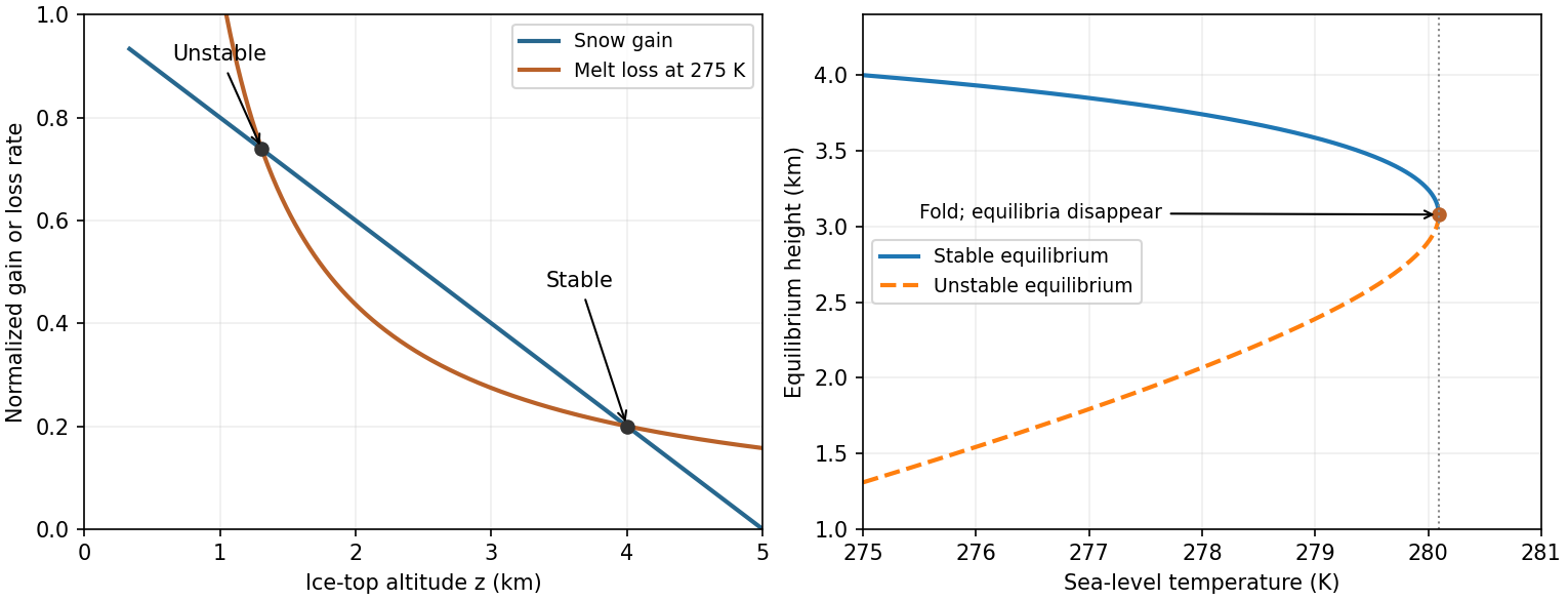
Write $s=T_s-273.15\mathrm{K}$ as the numerical sea-level Celsius temperature in degrees Celsius, and use the same degree increments for $\Gamma z$. The model's top temperature is $T_C=s-\Gamma z$. For positive $\alpha$ its intended cold-ice branch has $T_C<0$, so the positive melt-loss magnitude and snow gain areThe model is singular at $z=s/\Gamma$ and is not a physical melting law across that boundary. On the relevant interval $s/\Gamma <z<1/\beta$, $L$ decreases hyperbolically and $A$ decreases linearly. Assume a fixed area and positive ice density, so increasing mass increases $z$: stability has the same sign as $F^{\prime }(z)$.

The equilibrium equation iswith rootsTwo distinct physical equilibria, one stable, exist providedThis combines a positive allowed interval with a strictly positive discriminant. At the larger root $F^{\prime }<0$ and small perturbations restore the ice cap; the smaller root has $F^{\prime }>0$ and is unstable. Sincea restoring local response requiresThis is the lower height bound from the stability derivative; the stable equilibrium itself is $z_{+}$. The minimum initial height for persistence, a different notion of threshold, is the unstable separator $z_{-}$: initial heights above it approach $z_{+}$, while lower heights lose ice and leave the model's cold branch. At equality in the discriminant condition the two equilibria merge, giving a marginal fold rather than a strictly stable ice cap.

Complete oxidation of $10^{12}\mathrm{kg}$ of carbon adds $n_C=10^{12}/(12\times 10^{-3})=8.33\times 10^{13}\mathrm{mol}$ of carbon dioxide. With atmospheric mass about $5.1\times 10^{18}\mathrm{kg}$ and mean air molar mass $28.97\times 10^{-3}\mathrm{kg}\mathrm{mo}{\mathrm{l}}^{-1}$, there are about $1.76\times 10^{20}\mathrm{mol}$ of air. The dry-air mole fraction, approximately the volume fraction, changes byIt is the carbon inventory that counts: oxidation adds oxygen to each molecule but does not change the number of carbon-containing molecules. Using $5.15\times 10^{18}\mathrm{kg}$ instead changes the estimate by only about one percent. The atmospheric constants are standard Earth estimates, not additional data read from a missing plot.^[ref]

Newton's first law says that a body retains uniform rectilinear motion, including rest as the zero-velocity case, unless impressed forces change that motion. Its physical content includes the existence of a common class of inertial frames: free bodies do not each require an unrelated frame chosen just to straighten their own trajectory. Uniformity refers to the inertial time parameter, and straightness to the spatial structure of those frames. Everyday slowing under friction is compatible with this claim because it involves an interaction, not an exception to inertia.

Newton's second law relates the impressed resultant force to change of momentum. In modern continuous-force notation,so for constant mass it becomes $m\mathbf{a}={\mathbf{F}}_{\mathrm{net}}$. An impulsive version is $\Delta \mathbf{p}=\int \mathbf{F}dt$. The change is directed along the impressed resultant, not necessarily along the body's current velocity. The original wording concerns change of quantity of motion; the differential equation is its modern continuous-time formulation.^[ref]

These are substantive physical claims only when mass, interactions and the inertial structure are constrained independently. If “force” merely abbreviates whatever equals $m\mathbf{a}$ in any arbitrarily chosen coordinates, the second law by itself predicts nothing. Actual applications combine the law with independently testable interaction laws, vector addition of forces, initial conditions and a specification of the inertial frames.

Within an already specified inertial frame, with constant mass, substituting zero resultant force into Newton's second law does give zero acceleration. In that limited mathematical sense, force-free uniform motion is a special case. The reason for retaining Newton's first law is that its physical role is broader than this substitution.

The second law does not, just by its algebra, identify the coordinate systems in which acceleration measures the response to physical interactions. A free body described in coordinates $x^{\prime }=x-\frac{1}{2}A{t}^2$ has ${\ddot{x}}^{\prime }=-A$, despite experiencing no impressed interaction. If the second law is restricted to inertial frames, the first law supplies a criterion for that restriction and asserts that a common inertial structure exists. If instead one introduces a fictitious force $-mA$ to preserve the equation in the accelerated coordinates, that coordinate-dependent bookkeeping should not be confused with a newly discovered physical interaction.

Nor can the first law simply be used as a circular definition in which “free” means “unaccelerated” and “inertial” means “whatever makes the chosen body free”. The framework requires empirical identification of interactions and a mutually consistent class of free-body trajectories. Removing an influence or improving isolation should make the same inertial description work for many bodies, not merely one fitted trajectory.

Thus the two laws have distinguishable jobs: the first articulates the force-free inertial background; the second quantifies departures caused by impressed forces. A modern axiomatization may build that background into its spacetime structure and then omit a separately numbered first law. That is a legitimate reorganization, but it incorporates the first law's content rather than obtaining all of it from the equation $\mathbf{F}=m\mathbf{a}$. Newton states the laws separately in the opening axioms.^[ref]

Showing that acceleration is unchanged by a uniform boost is necessary, but it is not enough to establish the Galilean covariance of Newton's second law. One must specify how time, positions, masses, forces and any background physical systems transform, and show that the actual force laws retain their form.

For a constant spatial rotation $R$, boost velocity $\mathbf{U}$ and translations, writeDifferentiation gives ${\mathbf{v}}^{\prime }=R\mathbf{v}-\mathbf{U}$ and ${\mathbf{a}}^{\prime }=R\mathbf{a}$. Assuming invariant inertial mass,Consequently the equation has the same form if the resultant physical force satisfies ${\mathbf{F}}^{\prime }=R\mathbf{F}$. For a pure boost, this reduces to ${\mathbf{F}}^{\prime }=\mathbf{F}$. More explicitly, if a force is represented by a function of positions, velocities and other physical data, those arguments and data must transform so that its primed value is $R$ times the old value. It is this condition on the complete dynamical model, not the typography of $\mathbf{F}=m\mathbf{a}$, that establishes covariance.

An instantaneous inverse-square interaction depending on the separation of two particles passes this test: their common boost cancels from the separation, and a rotation rotates the force vector. A resistance law $\mathbf{F}=-\zeta (\mathbf{v}-\mathbf{u})$ also passes when the medium's velocity $\mathbf{u}$ transforms with the body. In contrast, keeping $\mathbf{F}=-\zeta \mathbf{v}$ in every boosted frame while silently resetting the same medium to rest changes the physical problem. That model has not been shown covariant by noting ${\mathbf{a}}^{\prime }=\mathbf{a}$.

Likewise, the full Maxwell equations are not made Galilean covariant merely because some equation of particle motion is written as force equals mass times acceleration. The covariance of a framework has to be checked together with its interaction laws. Newton's own Corollary V expresses the corresponding equivalence of uniformly translating, nonrotating systems for the mechanics under consideration.^[ref]

A white dwarf is a compact stellar remnant supported primarily by electron degeneracy pressure, radiating stored thermal energy rather than sustained main-sequence fusion. At zero-temperature leading order, filling electron momentum states gives $n_e=p_F^3/(3{\pi }^2{\hslash }^3)$ and $P=p_F^5/(15{\pi }^2{\hslash }^3{m}_e)$. Fully ionized hydrogen mass fraction $X$, with other nuclei approximately one electron per two nucleons, implies $n_e=(1+X)\rho /(2m_u)$. ThereforeThis is an $n=3/2$ polytrope. Solving hydrostatic structure with a zero-pressure surface gives $R=2.357K_1(1+X{)}^{5/3}{M}^{-1/3}/G$; the numerical factor uses ${\xi }_1=3.65375$ and $-{\xi }_1^2{\theta }^{\prime }({\xi }_1)=2.71406$ of that Lane-Emden solution. Thus $R\propto M^{-1/3}$. For $X=0$, $M=M_{\odot }$, $R$ is about $9\times 10^3$ km. A uniform-density scaling gives the same mass dependence but a different order-one coefficient and should be identified as such.

Independently, $R/R_{\odot }=\sqrt{0.056}(T_{\odot }/25000{)}^2\simeq 0.0126$, or about $8.8\times 10^3$ km. Agreement is good at this level; relativistic degeneracy becomes relevant for accurate modeling near one solar mass and eventually invalidates an unlimited nonrelativistic mass-radius law.

The 21.1 cm line is neutral hydrogen's hyperfine spin-flip transition, observed with radio telescopes and interferometers in the cool/warm neutral gas disk, often beyond the bright stellar disk. The mean wavelength gives $z=22.0/21.1-1\simeq 0.0427$ and, using the stated low-redshift Hubble approximation, $d\simeq 180$ Mpc. A 16-arcsecond angular radius gives $R\simeq 14$ kpc. For a thin circular disk, $\cos i=8/32$, so $i\simeq 75.5^{\circ }$ from face-on.

The original spectrum reaches roughly 21.98 and 22.02 cm: $v_{\mathrm{los},\max }\simeq c(0.02/22.0)\simeq 273$ km s${}^{-1}$. Deprojecting gives $\boxed{v_{\max }\simeq 282\mathrm{km}{\mathrm{s}}^{-1}}$. A spherical dynamical estimate $M(<R)\simeq v^{2}R/G$ gives $\boxed{M\sim 2.6\times 10^{11}{M}_{\odot }}$. A thin massive disk is not spherical: its exact rotation-to-total-mass coefficient depends on radial mass profile. The no-exterior-matter assumption does not uniquely fix that coefficient, so the quoted result is the conventional order-of-magnitude dynamical estimate. Cosmological luminosity and angular-diameter distances differ at this redshift; the source's simple Hubble-distance convention is being used consistently.

The low-redshift distance gives modulus about 36.28, so $M_V\simeq -20.28$ and $\boxed{L_V\simeq 10^{10}{L}_{\odot }}$. A stellar mass-to-light ratio of order one to a few would imply only $10^{10}$–several $10^{10}{M}_{\odot }$ in stars, below the dynamical estimate. Gas and a dark component can supply additional mass; the precise stellar estimate requires a population-dependent mass-to-light ratio and extinction correction.

An exponential luminous disk has most of its mass within a few scale lengths. Outside that concentration a mass-traces-light model tends toward a declining, approximately Keplerian speed, not an extended flat curve. Adding a spatially extended mass distribution explains the mismatch more naturally than merely rescaling the same concentrated light profile.