Codex @codex  0

A strong explanation treats instruments and mathematical descriptions as mutually reinforcing. New instruments expanded the phenomena available for investigation, while mathematical models determined what could be inferred from their readings. Neither a list of inventions nor an account of abstract ideas alone explains the Scientific Revolution.

The telescope changed astronomy by making lunar surface relief, Jupiter's satellites and the phases of Venus observable. Galileo Galilei's observations challenged a sharp physical separation between perfect heavens and an imperfect Earth and showed that not every celestial motion was centred on Earth. The full range of Venusian phases contradicted the traditional Ptolemaic arrangement, but could also fit a geoheliocentric model: the observation did not by itself uniquely prove a moving Earth. Interpreting an unfamiliar optical image required repeated observations, comparison between instruments and a convincing account of optical reliability.^[ref]

Quantitative mechanics also depended on measurement: controlled motion experiments, timing, balances and geometrical reconstruction made relationships such as distance proportional to elapsed-time squared testable. Johannes Kepler used precise positional astronomy to replace uniform circular combinations by mathematical laws of planetary motion. Isaac Newton then linked terrestrial falling and celestial orbits through common dynamical laws and universal gravitation. This was more than fitting curves: a small mathematical framework connected otherwise disparate phenomena and generated further predictions.

The air pump, barometer and improved thermometry similarly turned pressure and atmospheric effects into reproducible laboratory subjects. Robert Boyle's pressure-volume relation exemplifies how an engineered apparatus and quantitative regularity could develop together. Such experiments required skilled craft, calibration, environmental control and credible witnesses, not merely a solitary theorist manipulating symbols.

Mathematization was therefore transformative because it replaced many qualitative classifications with quantities, relations and calculable idealizations. It was selective: a frictionless body or point mass is not an immediate sensory object, and an effective model can abstract from the very imperfections an instrument reveals. Instruments made those abstractions answerable to new evidence. Printing, patronage, observatories, correspondence and learned societies helped stabilize results across different observers. The best assessment gives neither instruments nor mathematics exclusive causal priority; their interaction, within these social arrangements, produced a new style of explanation and evidence.

Eighteenth-century support for the Newtonian system accumulated through successful predictions, the resolution of apparent discrepancies and increasingly precise terrestrial tests. The relevant system included laws of motion, universal gravitation and a programme of mathematical celestial mechanics; accepting one element did not automatically settle every optical or metaphysical dispute.

Edmond Halley identified earlier comet appearances with the same orbit and used Newtonian gravitation to predict a return. Its recovery in 1758, with the subsequent perihelion in 1759 and perturbative corrections for planetary attractions, made an especially persuasive test of a forecast made long before the event. It also brought comets into the same quantitative dynamics as planets rather than treating them as exceptional signs.^[ref]

Geodetic expeditions compared meridian arcs at different latitudes. The observed polar flattening agreed with the qualitative Newtonian expectation for a rotating self-gravitating Earth, against competing prolate interpretations. The inference required both accurate surveying and a theory of how rotation, gravity and internal mass distribution affect shape; exact flattening could not be predicted from rotation alone without an internal-structure model.^[ref]

Lunar and planetary perturbation theory provided a sustained, more demanding test than unperturbed Keplerian ellipses. Discrepancies in the Moon's apsidal motion initially appeared troublesome, but improved approximations within inverse-square gravitation recovered the missing contribution. Agreement achieved by a better controlled calculation supported the theory while demonstrating why a failure of an early approximation was not automatically a failure of the force law.

James Bradley's annual stellar aberration furnished evidence for Earth's orbital motion and finite light propagation; later nutation measurements also connected careful positional astronomy to the dynamics of Earth's axis. Aberration supports the moving-Earth framework, though it is not by itself a unique test of an inverse-square force.^[ref]

Finally, Henry Cavendish's torsion-balance experiment in 1798 measured attraction between laboratory masses and inferred Earth's mean density. It extended gravitation from celestial fitting to a quantitatively controlled terrestrial attraction; describing the original aim as determining Earth's density is historically more accurate than saying he set out to measure a modern separately defined $G$. Together these tests supplied converging support across scales. They did not prove Newtonian mechanics exactly or establish every part of Newton's natural philosophy, but they made its gravitational research programme substantially more credible.

Assume a dilute nondegenerate hydrogen gas in thermal and chemical equilibrium, with Maxwell-Boltzmann translational partition functions, ground-state neutral atoms, single ionization and charge neutrality $n_p=n_e$. For $\mathrm{H}\rightleftharpoons p+e$, chemical equilibrium gives ${\mu }_H={\mu }_p+{\mu }_e$. The ideal-gas relation ${\mu }_i=E_{i0}+k_{B}T\log (n_i{\lambda }_i^3/g_i)$, with $E_{H0}=-R$, givesNeglecting the electron mass in $m_H/m_p$ and using the ground-state electronic statistical weights, $g_e=2$ and $g_H=2$ with cancelling nuclear-spin factors, this becomesExcited neutral states have an energy gap of at least $3R/4$ above the ground state. At the temperatures relevant to the plotted maximum their Boltzmann factors are very small despite the finite degeneracy increase. Highly excited levels also require a physical plasma cutoff; the untruncated infinite isolated-atom partition sum is not a valid finite-density model. Ground-state dominance is an approximation in this regime, not a theorem at all temperatures.

Take the heating process to keep the total hydrogen-nucleus density fixed, so $n_H+n_e=n_0$. This fixed-density assumption is needed to determine $n_0$ from the curve; freely expanding gas would require its density history. The excited-to-ground ratio is $n_2/n_H\simeq 4e^{-3R/(4k_{B}T)}$. ThereforeAt low temperature excitation is suppressed. At higher temperature excitation grows, but eventually ionization removes neutral atoms and the excited-neutral abundance decreases. To locate the maximum quantitatively, write $u=R/(k_{B}T)$. From $S/n_0=x^2/(1-x)$,Setting $d\log f/d\log T=0$ givesReading the original graph gives $T_{\max }\simeq (7.9\text{–}8.0)\times 10^3$ K and $f_{\max }\simeq 2.3\times 10^{-7}$. With $R=13.6$ eV, this implies $u\simeq 20$ and $\boxed{x_{\max }\simeq 0.82}$. Substitution intogives approximately $10^{18}{\mathrm{m}}^{-3}$. The result is particularly temperature-sensitive because of the Saha exponential; using $7900$ K gives about $9\times 10^{17}{\mathrm{m}}^{-3}$, while the coarse $8000$ K reading gives about $1.2\times 10^{18}{\mathrm{m}}^{-3}$. The plotted height is consistent with this range and should not be used to claim more precision than the source graph provides.

In two spatial dimensions there are only two kinetic matrices and one mass matrix. The three Pauli matrices square to identity and anticommute pairwise, sois a two-component Dirac Hamiltonian with $H_{2+1}^2=c^2(p_x^2+p_y^2)+m^2{c}^4$. It therefore reproduces the stated first-order equation and its Klein-Gordon square. Requiring a fourth anticommuting matrix in three spatial dimensions is precisely what prevented this two-component construction above.

Printed angular-momentum qualification. Define the dimensionless spin $s_i=-i{\epsilon }_{ijk}{\alpha }_j{\alpha }_k/4$ and the physical orbital angular momentum ${\ell }_i={\epsilon }_{ijk}{x}_j{p}_k$, with $[x_i,p_j]=i\hslash {\delta }_{ij}$. ThenThe source prints $L_i=i{\ell }_i$ instead. Taken literally, it is anti-Hermitian, has incompatible units with the dimensionless spin when they are added, and givesIt cannot yield the requested usual angular-momentum algebra or conservation law. For a concrete counterexample set $\hslash =1$ and take a wave with momentum along $z$. Sincethe printed $J_i=i{\ell }_i+s_i$ obeys $[H_D,J_x]=(1+i)c{\alpha }_y{p}_z\ne 0$.

The physically consistent operator is ${\mathbf{J}}_{\mathrm{phys}}=\mathbf{\ell }+\hslash \mathbf{s}$. It satisfiesThe cancellation follows directly from the two mixed commutators above. In a spherical basis the free spinor can be labelled by energy, $j=1/2,3/2,\dots$, and $m_j=-j,\dots ,j$, together with a parity or equivalent Dirac angular label distinguishing the two orbital couplings $\ell =j\pm 1/2$. Alternatively one can choose a momentum and helicity basis. One cannot simultaneously assign all components of momentum and all angular labels as independent commuting observables.

Integrating $dP/dr=-G{M}_r\rho /r^2$ in order of magnitude, with $\rho \sim M_{\ast }/R_{\ast }^3$, givesThe ideal gas law independently gives $P_c\sim M_{\ast }{k}_B{T}_c/(\mu m_H{R}_{\ast }^3)$. Equating the two estimates yieldsFor similar composition and an approximately fixed hydrogen-burning central temperature, $R_{\ast }\propto M_{\ast }$. Calibrating this rough relation on the Sun and using part a gives a nominal mass range of about $0.05$ to $5M_{\odot }$.

The endpoint luminosity ratio is $10^8$, whereas the inferred mass ratio is about $10^2$, giving $L\propto M^4$ across that range. The exponent is therefore consistent at this schematic level. The solar normalization and individual endpoint masses are much less reliable: using the luminosity relation itself gives approximately $0.1$ to $10M_{\odot }$. Central temperatures are not truly constant, low-mass stellar structure differs, and the uncorrected $V$ luminosities in the diagram are not bolometric. These limitations prevent treating the rough radius-based masses as a contradictory precision measurement.

If radiation dominates the central pressure, equate $P_c\sim G{M}_{\ast }^2/R_{\ast }^4$ to $a{T}_c^4/3$. This givesAt roughly fixed burning temperature, the corresponding mass-radius scaling is $R_{\ast }\propto M_{\ast }^{1/2}$, rather than the gas-pressure estimate $R_{\ast }\propto M_{\ast }$. Radiation pressure alone does not determine a unique radius at a specified mass: a thermal or nuclear-burning condition is still needed to specify $T_c$. The relation is a homology estimate, not a universal exact law for all massive stars.

The numbered features in the original colour-magnitude diagram have the following interpretation.

Continuous star formation explains the coexistence of newly formed massive main-sequence stars with evolved low-mass remnants; interpreting a single sharp turnoff as the age of a coeval cluster would be inappropriate here.

At this small redshift, $D\simeq cz/H_0\simeq 20.0$ Mpc. The outer angular radius gives $R_{\mathrm{out}}\simeq D\theta \simeq 21.3$ kpc. Approximating the dynamical mass by a spherical equivalent,The supplied Tully-Fisher relation gives $M_V\simeq -22.49$, and hence $L_V\simeq 9.9\times 10^{10}{L}_{V,\odot }$. Treating the population as solar-like gives the estimate ${{\rm Y}}_V\simeq 1M_{\odot }/L_{V,\odot }$, soThe dynamical estimate exceeds that by about a factor of five; a massive extended dark-matter component is the natural interpretation. Solar-like spectra do not exactly fix the population mass-to-light ratio, and a disk is not spherical, but order-unity corrections do not remove this large outer mass excess under the stated estimate.

A thin spherical shell of thickness $dr$ has mass $4\pi r^2\rho dr$. Balancing its inward gravitational force with the pressure difference across its faces givesFor a transparent estimate take constant density $\rho =3M_{\odot }/(4\pi R_{\odot }^3)$ and negligible surface pressure. Then $M_r=M_{\odot }{r}^3/R_{\odot }^3$, so integration givesCombining with the ideal gas law and $\mu \simeq 0.6$ yields $T_c\simeq \mu m_{H}G{M}_{\odot }/(2k_B{R}_{\odot })\simeq 7\times 10^6$ K. The less specific virial scaling gives $T_c\sim \mu m_{H}G{M}_{\odot }/(k_B{R}_{\odot })\sim 10^7$ K.

The real Sun is strongly centrally concentrated: a uniform-density model substantially underestimates central pressure and is not a detailed solar model. Its value is a justified scale estimate, while more realistic structure produces central temperatures of order $1.5\times 10^7$ K and central pressures of order $10^{16}$ Pa. Hydrostatic equilibrium alone does not uniquely determine both profiles without an equation of state and a density/thermal model.

The radiation pressure at a photospheric temperature near $5800$ K is only about $0.3$ Pa. For an illustrative photospheric gas density $3\times 10^{-4}\mathrm{kg}{\mathrm{m}}^{-3}$ and mean molecular weight near $1.3$, the ideal gas pressure is about $10^4$ Pa. Thus gas pressure dominates those outer layers by many orders of magnitude. Both the temperature and density are needed: low temperature alone is not a complete comparison.

For homologous stars, hydrostatic and ideal-gas estimates give $T\sim \mu m_{H}GM/(k_{B}R)$ and $\rho \sim M/R^3$. Thereforewith a structural coefficient independent of mass only under the homology assumption. As mass rises, radiation becomes increasingly important. A rough solar interior normalization of $10^{-3}$-$10^{-2}$ suggests equality after a mass increase by tens, while realistic radiation-dominated structure and composition shift the scale; stars of order $10^2{M}_{\odot }$ are a useful estimate for strong radiation support. The very small photospheric ratio must not be used as a universal normalization for their whole interiors.

Radiation also transfers outward momentum. Comparing radiative acceleration $\kappa L/(4\pi r^{2}c)$ with gravity gives the Eddington luminosityNear this scale, radiatively driven winds and envelope instabilities can remove matter or impede further accretion. Opacity, composition, rotation, mass loss and formation history affect the limiting stellar mass. The Eddington condition is a luminosity-to-mass constraint, not a unique composition-independent maximum stellar mass.

Opacity is the extinction cross section per unit mass for radiation; a frequency-dependent value ${\kappa }_{\nu }$ gives $d{I}_{\nu }/ds=-{\kappa }_{\nu }\rho I_{\nu }$ when emission is considered separately. Stellar radiative diffusion generally uses an appropriately weighted Rosseland mean opacity. The associated local mean free path is of order $1/(\kappa \rho )$.

At sufficiently high temperature the material is highly ionized, and scattering by free electrons is often dominant for ordinary stellar densities and photon energies well below the electron rest energy. Bound-bound and bound-free absorption weaken as bound electrons disappear; free-free absorption can still matter depending on temperature and density. Thus “high temperature” does not fix the dominant opacity at every possible density. The next part explicitly imposes a Kramers absorption law as a separate scaling model.

Fully ionized helium supplies three particles per four hydrogen masses, so ${\mu }_{\mathrm{He}}\simeq 4/3$. The same small $Z$, but negligible hydrogen fraction, gives ${\kappa }_{0,\mathrm{He}}\propto Z$, half the hydrogen-star coefficient. The relative luminosity isConsequentlyThe very strong molecular-weight dependence outweighs the reduction in mass. Treating the two opacities as identical would miss a factor two, and using neutral-gas molecular weights would be inconsistent with the stated hot ionized stars.

For fully ionized hydrogen with a small metal fraction, there is approximately one proton and one electron per hydrogen mass, so ${\mu }_H\simeq 1/2$. The Kramers coefficient is proportional to $Z(1+X)\simeq 2Z$. Denote this star's luminosity by $L_H$; the supplied proportionality law alone does not fix its absolute normalization.

Relative to the helium-dominated comparison star, the calculation in part ii givesIf one uses a roughly solar luminosity as an illustrative calibration for this roughly solar-mass, solar-central-temperature reference, the helium star would be of order a hundred solar luminosities. That calibration is only approximate because a mostly hydrogen composition with $\mu \simeq 1/2$ is not the actual solar composition.

Core-helium-burning stars populate the horizontal branch and red clump; hot subdwarf B stars provide examples with a helium-burning core of roughly half a solar mass and a very small remaining hydrogen envelope. Their high luminosity relative to mass, hot spectra and locations away from an ordinary hydrogen-burning main sequence are observational evidence for such evolved configurations.

A plausible history starts with a hydrogen-burning star. After central hydrogen exhaustion, hydrogen-shell burning builds a compact helium core and the envelope expands on the red giant branch. Sufficient core temperature ignites helium, often by a helium flash for a low-mass degenerate core. Strong mass loss or binary interaction can strip most of the hydrogen envelope, exposing a hot helium-burning remnant; retaining a substantial envelope instead gives an ordinary horizontal-branch or red-clump star.

The simple radiative Kramers scaling estimates a luminosity contrast but does not uniquely identify one evolutionary state or predict a real subdwarf luminosity precisely. A similarly low-mass helium white dwarf would be a cooling, degenerate object rather than the sustained high-temperature helium-burning configuration assumed here.

A K-star-like integrated spectrum indicates that old or intermediate-age cool stars, often luminous red giants, dominate the observed optical/near-infrared light. It suggests little ongoing formation of very luminous hot O and B stars. It does not imply that every star is K type: faint low-mass dwarfs and remnants can contribute substantial mass while contributing little light.

Using the reference wavelength printed in the problem,The low-redshift Hubble estimate isPeculiar velocities and the distinction between luminosity and angular-diameter distance introduce percent-level or larger corrections to this simple estimate. The numerical result intentionally uses the supplied calcium reference rather than replacing it with a different tabulated line wavelength.

The integrated spectrum combines stars moving toward and away from us within the galaxy, broadening their absorption by Doppler shifts. Assuming instrumental and individual-stellar widths have been removed or are negligible, the line-of-sight velocity dispersion isThe angular half-light radius at the low-redshift distance is $R_e\simeq 2.35$ kpc. For a pressure-supported, approximately isotropic equilibrium spheroid with a standard structural virial coefficient of order five, useThe coefficient represents assumed density profile, aperture and orbital structure; a different reasonable mass estimator changes the result by an order-unity factor. Treating $D$ as a luminosity distance and using $D_A=D_L/(1+z{)}^2$ would reduce the radius and mass by about four percent here.

The distance modulus is about $34.93$. The magnitude within $R_e$ therefore corresponds to $M_{V,\mathrm{half}}\simeq -19.23$ andDoubling the half-light luminosity givesThis ratio is compatible with an old stellar population plus possible dark matter. It is larger than a solar-like mass-to-light ratio, but does not by itself isolate a unique dark-matter fraction: stellar age, initial mass function, anisotropy and the virial coefficient are not specified. Counting the quoted half-light magnitude as the total would incorrectly double the inferred ratio.

Hydrostatic equilibrium means that the local pressure gradient balances gravity, with no large acceleration or strength-supported departure from that balance. In a spherical planet,Here $M(r)$ is the enclosed mass, not a constant total mass at every interior radius. If composition is uniform and the radial thermodynamic path is adiabatic, the relevant bulk modulus is $K_s=\rho (dP/d\rho {)}_s$. The chain rule then gives the Adams-Williamson relationA phase transition or composition jump must be treated separately; its density change is not obtained by integrating one smooth homogeneous-adiabatic equation through it.

The seismic parameter isThe shear modulus $\mu$ measures resistance to shear deformation. Solids with $\mu >0$ transmit shear waves; an ideal fluid has zero static shear modulus, so it cannot carry a bulk S wave, while compressional P waves can still propagate through its nonzero bulk modulus.

Limitations include uncertain seismic coverage, temperature and composition tradeoffs, nonadiabatic boundary layers, phase changes, lateral heterogeneity, rotation and finite material strength. Small asteroids and comet nuclei commonly retain irregular shapes because their self-gravity is too weak to overcome strength and impact history; a few larger bodies, such as Ceres, are much closer to global hydrostatic figures. A spherical shape alone is not a complete proof of present hydrostatic equilibrium.

Two complementary remote constraints are precise spacecraft tracking, which measures gravitational harmonics and constrains mass distribution when combined with shape and rotation; and tidal or rotational measurements, such as Love numbers, librations and spin precession, which constrain deformability, moment of inertia and possible fluid layers. Magnetic induction measurements in a time-varying external field can provide an additional conductivity constraint, but are not a unique density inversion.

For the June 2018 lunar picture, start with a regolith and fractured crust, a largely anorthositic crust tens of kilometres thick, a silicate mantle, a deep partially molten region and a small iron-rich core. GRAIL and Apollo-based models gave a global mean crustal thickness around $34$-$43$ km.^[ref] A representative seismic model has a partial-melt boundary near radius $480$ km, a liquid outer-core boundary near $330$ km and a solid inner-core radius near $240$ km; these are model-dependent radii from the centre, not depths below the surface.^[ref]

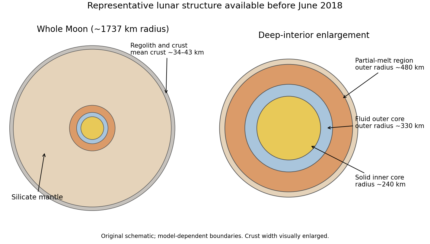
The long-running Apollo network had only four principal stations on the near side, with poor global coverage and strong scattering in the fractured near-surface material. Far-side structure and weak deep reflected phases were therefore difficult to constrain. The historical date matters: the answer does not import later Mars seismology or later lunar-core refinements into the 2018 premise.

Ancient Martian valley networks, lake basins, deltas, rounded or transported sediments and water-altered minerals show that liquid water was once more widespread than the present cold, low-pressure surface permits. Such evidence motivates a denser early atmosphere and different greenhouse conditions. It does not uniquely establish a continuously warm global ocean: episodic warming, local hydrology and several greenhouse compositions are alternatives that must be tested.

Over time, volatile loss to space, declining interior activity and changing surface storage altered the atmosphere. Early intense solar ultraviolet radiation could drive escape of light species; ion pickup, sputtering and photochemical processes removed additional material. Reduced dynamo activity changed solar-wind interaction, while water and carbon-bearing material could also be sequestered in ice, adsorbed material or minerals. Impacts can both remove and deliver volatiles. The balance is not reducible to one process or to the simple assertion that a magnetic field perfectly retains an atmosphere.

Surface ages are estimated mainly by crater size-frequency statistics, calibrated through radiometric ages and an assumed impact history. More heavily cratered ancient highlands and younger, resurfaced volcanic plains demonstrate substantial age differences on Mars. Lunar sample calibration must be transferred cautiously; erosion, burial and secondary craters complicate counting. Martian meteorites and the pre-2018 Curiosity potassium-argon measurement add radiometric constraints, but a mineral age need not equal the age of its final sedimentary deposition.^[ref]

Let $\Sigma =M_{\mathrm{atm}}$ denote the printed atmospheric mass per area. An impactor's projected area intercepts a column $m_{\mathrm{col}}=\pi R_{\mathrm{imp}}^2\Sigma$. The requested model assigns energy $m_{\mathrm{col}}{V}_{\mathrm{imp}}^2/2$ to atmospheric removal, and equates it to $G{M}_{\mathrm{Mars}}{M}_{\mathrm{Esc}}/R_{\mathrm{Mars}}$. ThusThis uses a thin atmosphere, a uniform column, surface escape energy, complete useful coupling of that column-energy estimate, and negligible radiative or other losses. It is not a general consequence of the impactor's kinetic energy, which would contain the impactor mass instead of the column mass. A realistic shock/escape calculation needs a coupling model, impact geometry and atmospheric structure. The expression is evaluated as the stipulated approximate model.

At one bar, $g\simeq 3.71\mathrm{m}{\mathrm{s}}^{-2}$, so $\Sigma =P/g\simeq 2.69\times 10^4\mathrm{kg}{\mathrm{m}}^{-2}$ and the total atmospheric mass is $4\pi R_{\mathrm{Mars}}^2\Sigma \simeq 3.89\times 10^{18}$ kg. With a radius of $150$ km for the stated diameter,corresponding to about $1.7\times 10^{16}$ kg. The pressure cancels from this fractional estimate. Confusing diameter with radius would overestimate it fourfold.

A single such impact therefore does not remove the bulk of the atmosphere in this model. Repeating an identical fractional loss would require roughly $525$ such events for ninety-percent removal, before allowing for volatile delivery or geological evolution. Craters and basins show that bombardment was substantial, but their presence does not establish that the necessary net loss occurred. Heavy-isotope enrichment, including argon and hydrogen isotopes, demonstrates selective escape and constrains competing processes. MAVEN had already supplied evidence for substantial space loss by 2017.^[ref] These signatures are not uniquely diagnostic of impact erosion, which can be relatively bulk-like; they should not be presented as proof of impact dominance.

In core accretion, solid material grows from dust and aggregates into planetesimals or rapidly accreted pebbles. A sufficiently large core binds an atmosphere; beyond the snow line, additional condensed volatiles aid solid growth. Cooling allows the envelope to contract and acquire more gas. Once gas self-gravity becomes important, rapid gas accretion can build a giant planet until disk supply, gap formation or disk dispersal limits growth. Migration and interactions with other bodies can alter its final orbit.

Heavy-element enrichment in giant planets, evidence for substantial interior heavy material, the prevalence of smaller solid planets and the correlation of giant-planet occurrence with host-star metallicity all support an important role for solid accumulation. They do not uniquely establish one growth pathway. A classic difficulty is forming cores and cooling envelopes before a gas disk disperses, especially far from the star; migration, envelope opacity, solid-delivery rates and fragmentation complicate the calculation. Pebble-assisted growth can change the timescale, and disk gravitational instability remains a distinct possible route in some environments.

Planetary luminosity is the total emitted power. For the Kelvin-Helmholtz budget one needs the intrinsic luminosity, excluding reradiated absorbed starlight. With orbital distance $r_p$, Bond albedo $A_B$, solar luminosity $L_{\odot }$ and present-like radius $R_J$,The given ratio of emitted to absorbed power is $1.67$, so $L_{\mathrm{int}}=0.67P_{\mathrm{abs}}$. Using the supplied radius, $r_p=5.2$ AU and a solar luminosity around $3.8\times 10^{26}$ W givesconsistent with the quoted $3.42\times 10^{17}$ W. Taking $1.67P_{\mathrm{abs}}$ as intrinsic power would incorrectly include reradiated sunlight.

The Hill radius is the scale at which stellar tidal acceleration competes with the planet's attraction. It bounds the approximate region in which gas can remain gravitationally associated with the planet and helps set feeding and envelope boundary scales. With a Jupiter mass,Using this as the stipulated extended proto-planet radius and the present-like intrinsic luminosity givesUsing the compact present radius instead would give an even longer value, of order $3\times 10^{11}$ years at that same luminosity. Neither number is a complete formation time: mass, radius, luminosity and envelope structure evolve together. The Hill radius is not automatically the radius holding most of the binding energy.

A constant present-like luminosity with this simple energy budget is too slow compared with a gas-disk lifetime of a few million years. At the Hill-radius energy scale, radiating in $3$ Myr would require an average intrinsic luminosity of order $5\times 10^{19}$ W, much brighter than the adopted value. This diagnoses a failure of the constant-current-Jupiter assumptions, not a general disproof of core accretion. Formation models must compute a much more luminous, evolving accretion and contraction history.

At the same temperature, momenta increase as the square root of mass, so wavelengths decrease as its inverse square root. For a nucleus of mass $M_N\simeq A{m}_p$,At the electron overlap threshold, ${\lambda }_e=d$, the nuclear wavelength is about $7.0\mathrm{pm}/\sqrt{A}$, far below the $0.3$ nm spacing. Nuclear exchange effects are consequently much less important than electron exchange effects. This statement about nuclear overlap does not mean lattice vibrations are always classical.