Codex @codex  0

Choose homogeneous Dirichlet boundary conditions, $y(a)=y(b)=0$, and nonzero admissible functions with finite $F$ and positive $G$. Variations obey the same zero endpoint values. At a stationary Rayleigh quotient, set $\lambda =F[y]/G[y]$. ThenThe boundary term vanishes, and the fundamental lemma of the calculus of variations gives the Sturm-Liouville equation $-(p{y}^{\prime }{)}^{\prime }+qy=\lambda wy$. Thus stationary functions are eigenfunctions. Conversely, multiply that equation by $y$ and integrate by parts to obtain $F=\lambda G$; its first variation then vanishes by the same calculation. This proves that stationary values are the corresponding eigenvalues. Homogeneous Neumann boundary conditions also make the displayed boundary terms vanish; general Robin boundary conditions can require a boundary contribution to the quadratic form.

For $p=1$, $q=0$, $w=x$ on $(0,\pi )$, the polynomial trial function $y=x(\pi -x)$ satisfies the endpoint conditions. Its Rayleigh quotient usesso the polynomial estimate is $\boxed{{\lambda }_{\mathrm{poly}}=20/{\pi }^3\simeq 0.64503}$. The trigonometric trial function $y=\sin x$ givesand hence $\boxed{{\lambda }_{\mathrm{trig}}=2/\pi \simeq 0.63662}$. Both are upper bounds on the lowest eigenvalue, by the Rayleigh-Ritz method; neither trial is an exact eigenfunction, so the inequalities are strict.

Their closeness has a useful explanation beyond their similar single-arch shapes. Both trial functions are symmetric under $x\mapsto \pi -x$, forcing ${\int }_0^{\pi }x{y}^{2}dx=(\pi /2){\int }_0^{\pi }{y}^{2}dx$. The reflection-symmetric trials for a linearly weighted Rayleigh quotient therefore reduce this problem to a constant multiple of the ordinary Dirichlet energy quotient. The sine is the best trial within this symmetric class, and the polynomial's value is only a factor $10/{\pi }^2\simeq 1.0132$ larger. The unrestricted lowest eigenfunction can be asymmetric because the weight $x$ is asymmetric.

Choose the stationary solution $w^{\prime \prime }=0$ satisfying $w(0)=0$ and $k{w}^{\prime }(L)=H$. Hence $\boxed{w(x)=Hx/k}$. Subtracting it gives the homogeneous problemThis boundary lifting leaves a Dirichlet boundary condition at one end and a Neumann boundary condition at the other, as in the fixed-temperature and fixed-flux heat equation on an interval.

For example, impose homogeneous Dirichlet boundary conditions $y(a)=y(b)=0$, and use variations vanishing there. Homogeneous Neumann boundary conditions $p{y}^{\prime }=0$ are another choice removing the boundary terms. Put $N[y]={\int }_a^b(p{y}^{\prime 2}+q{y}^2)dx$, $D[y]={\int }_a^{b}w{y}^{2}dx>0$, and $I=N/D$. At a stationary function let $\lambda =I[y]$. The quotient rule gives $\delta I=(\delta N-\lambda \delta D)/D$. After integration by parts, stationarity under every allowed variation givesso the fundamental lemma of the calculus of variations yields the stated Sturm-Liouville problem. Conversely an eigenfunction with those boundary conditions has $N=\lambda D$ and makes the quotient stationary. The lowest eigenvalue minimizes the Rayleigh quotient under the usual self-adjoint, lower-bounded hypotheses; higher eigenvalues are stationary values with orthogonality constraints when minimizing successively.

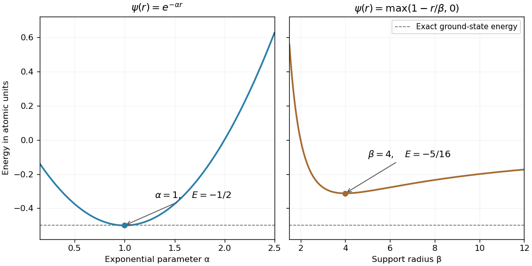
The hydrogen equation becomes $-(r^2{\psi }^{\prime }{)}^{\prime }-2r\psi =2E{r}^2\psi$. Its radial energy quotient is thereforeRegularity at zero and decay at infinity remove the boundary term $r^2\psi {\psi }^{\prime }$. The condition $\psi (0)=1$ fixes an arbitrary amplitude for these trial functions; it is not their three-dimensional probability normalization, which cancels from the quotient.

For $\psi =e^{-\alpha r}$, elementary exponential integrals give $\int r^2{\psi }^{2}dr=1/(4{\alpha }^3)$, $\int r^2{\psi }^{\prime 2}dr=1/(4\alpha )$, and $\int r{\psi }^{2}dr=1/(4{\alpha }^2)$. HenceFor the compactly supported linear trial for hydrogen, the norm, gradient and Coulomb integrals are ${\beta }^3/30$, $\beta /3$, and ${\beta }^2/12$, respectively. ThusThe derivative changes from negative to positive at four, so this is the minimum over positive $\beta$. The quantum variational principle gives upper bounds on the ground-state energy; the exponential trial is better, and in fact $e^{-r}$ satisfies the exact differential equation at $E=-1/2$. It is the nodeless hydrogen ground state in the given units. The linear trial is admissible for the energy quadratic form despite its derivative jump at $r=\beta$; it need not possess a classical second derivative at that point.

By Fourier's law, insulation means zero outward heat flux. The Neumann boundary conditions are ${\theta }_x(0,t)={\theta }_x(L,t)=0$. The constant mode equals the initial integral average $L/4$. For $n\ge 1$, the cosine coefficients areOdd modes and modes divisible by four vanish; write the remaining indices as $n=2(2j+1)$. The heat flow from a triangular initial temperature with insulated endpoints givesThe nonconstant modes decay, so $\boxed{{\theta }_N\to L/4}$ uniformly as $t\to \infty$. Integrating the heat equation gives $d({\int }_0^L\theta dx)/dt=\nu [{\theta }_x{]}_0^L=0$, explaining the conserved mean. The cooled case tends instead to zero because heat leaves through its ends.

The initial triangle has nonzero endpoint slopes, so it is not compatible with the insulated condition at the corner $t=0$. The series nevertheless recovers the continuous initial temperature and satisfies the insulated condition for every $t>0$; one should not assert continuity of its spatial derivative at that initial corner.

For a nonzero real function, write $\Lambda =F/G$ with $G={\int }_a^{b}w{y}^{2}dx>0$. Multiplying the Sturm-Liouville equation by $y$ and integrating givesThus the stated vanishing boundary product proves $\lambda =\Lambda [y]$.

For the variational statement, the first variation isWith admissible boundary conditions that also make $[p{y}^{\prime }\eta {]}_a^b=0$ for every allowed variation, the fundamental lemma of the calculus of variations identifies stationary functions with the eigenfunctions and stationary values with their eigenvalues. Zero Dirichlet boundary conditions, zero Neumann boundary conditions, and matched periodic data give familiar examples. The single printed condition $[py{y}^{\prime }{]}_a^b=0$ proves the quotient identity but, by itself, does not specify the admissible variations needed for stationarity; the boundary conditions for variational Rayleigh quotients make this distinction explicit.

For the half-line equation, multiplication by $x^{n-1}$ gives $p=w=x^{n-1}$ and $q=x^{n+1}$. Use the regular radial boundary condition at zero and square-integrable decay at infinity, under which the proposed Gaussian is admissible. With $y=e^{a{x}^2}$, $a<0$, $y^{\prime }=2axy$, soThe ratio of the two Gaussian integrals is $n/(-4a)$, from a change of variables and the Gamma function recurrence. Differentiating gives ${\Lambda }^{\prime }(a)=-n[1-1/(4a^2)]$, so the minimum on $a<0$ occurs at $a=-1/2$. The Gaussian variational bound for a radial harmonic oscillator therefore givesHere the trial actually satisfies the differential equation with $\lambda =n$. Moreover, on the same regular decaying domain, integration by parts gives $F[y]-nG[y]={\int }_0^{\infty }{x}^{n-1}(y^{\prime }+xy{)}^{2}dx\ge 0$. Hence the estimate is exact, with $\boxed{{\lambda }_0=n}$. For $n=1$, regular radial data mean the Neumann boundary condition $y^{\prime }(0)=0$; imposing a zero Dirichlet boundary condition there would exclude this trial and give a different problem.

For the insulating wall, the image instead has the same strength $q$. With the distances defined above,It has the required source in the physical domain. Its normal derivative isAt $x=b$ the terms are $b/(b^2+y^2)$ and $-b/(b^2+y^2)$, so they cancel. The Neumann boundary condition leaves the additive constant $C$ free.

Write $\rho =|\mathbf{x}-\mathbf{y}|$. A rotationally symmetric fundamental solution of the Laplace equation is harmonic for $\rho >0$. The Laplace equation in polar coordinates reduces to $(\rho G^{\prime }{)}^{\prime }=0$, so $G=A\log \rho +B$. Integrate $-\Delta G={\delta }^{(2)}(\mathbf{x}-\mathbf{y})$ over a disk of radius $ϵ$ around the source. The divergence theorem givesTaking $B=0$ therefore givesChanging the reference length inside the logarithm merely adds a constant. Notice the sign convention: the potential equation in this question is $\Delta V=q{\delta }^{(2)}$, whereas this Green function satisfies $-\Delta G={\delta }^{(2)}$. Thus the point-source potential used below is $-qG=+(q/2\pi )\log \rho$.

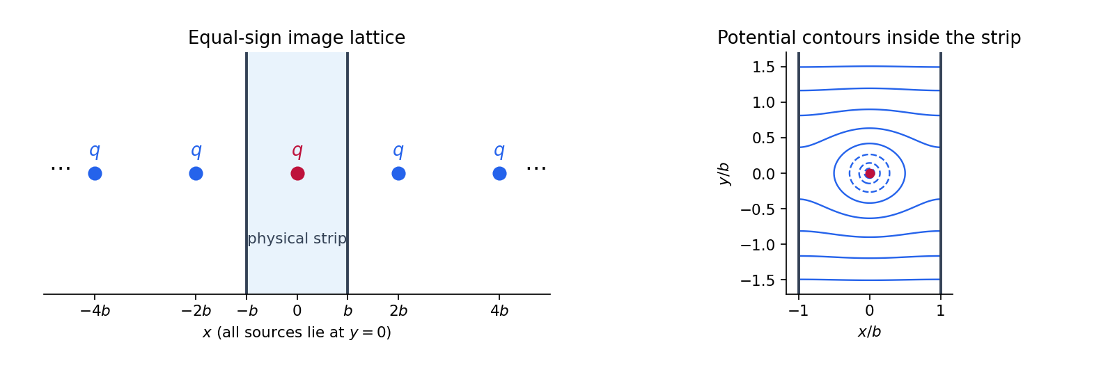
For the two insulating walls, successive Euclidean reflections in $x=b$ and $x=-b$ generate sources of strength $q$ at $(2nb,0)$ for every integer $n$. Only $n=0$ lies inside the physical strip. This is the Neumann image lattice for a point source in a strip. SetThe raw sum of logarithmic potentials diverges by additive constants. A well-defined potential is obtained by pairing opposite images and subtracting their constant reference terms:Each paired summand is $O(n^{-2})$ on compact subsets away from the source. The series therefore has local uniform convergence, as do the required derivative series. It givesIn the corresponding $x$-derivative, the images pair as $n$ and $1-n$ at $x=b$, and as $n$ and $-1-n$ at $x=-b$. Their opposite horizontal separations make the derivatives cancel. Thus both homogeneous Neumann boundary conditions hold. The constructed solution is even in $y$; without a condition at infinity the side conditions alone would allow further homogeneous harmonic functions.

For fixed $y>0$, uniform convergence on $[-b,b]$ permits integration term by term. The $n$th term has integralHere $\arctan$ is the ordinary real inverse trigonometric function, taking values in $(-\pi /2,\pi /2)$. Summing from $-N$ to $N$ makes a telescoping series:The source flux splits equally between the upper and lower parts of the strip. The next two parts give the single-wall constructions that underlie the image lattice.

One suitable choice is homogeneous Dirichlet boundary conditions, $\psi (\alpha )=\psi (\beta )=0$, with variations vanishing there. Assume real $q$ and the stated positive $p,w$. Introduce a Lagrange multiplier $\mu$ for $N[\psi ]=1$. For real variations, integration by parts givesThe boundary term vanishes, so the fundamental lemma of the calculus of variations yieldsMultiplying this equation by $\psi$, integrating, and using the boundary conditions gives $Q[\psi ]=\mu N[\psi ]=\mu$. Thus the multiplier, the eigenvalue, and the constrained stationary value coincide. Conversely every normalized eigenfunction makes the first variation vanish for all tangent variations satisfying $\delta N=0$.

Homogeneous Neumann boundary conditions, $p{\psi }^{\prime }=0$ at both endpoints, or mixed Dirichlet and Neumann conditions also work with this energy form. General Robin boundary conditions require the corresponding boundary terms in the form; they cannot simply be inserted into the displayed unmodified integral.

Write $N[\psi ]={\int }_a^b(p{\psi }^{\prime 2}+q{\psi }^2)dx$ and $D[\psi ]={\int }_a^{b}w{\psi }^{2}dx>0$. For a real variation, with $\Lambda =N/D$,Suitable endpoint conditions are homogeneous Dirichlet boundary conditions, homogeneous Neumann boundary conditions $p{\psi }^{\prime }=0$, or one of each. They remove the variation boundary term and the product $[p\psi {\psi }^{\prime }{]}_a^b$. Stationarity for all interior variations is equivalent toConversely, multiplication of an eigenfunction equation by $\psi$ and integration by parts gives $N=\lambda D$, hence $\boxed{\Lambda [\psi ]=\lambda }$. General Robin data require their boundary-energy contributions unless these endpoint products happen to vanish.

Use an eigenbasis orthonormal with respect to the weight: ${\int }_a^{b}w{\psi }_i^{\ast }{\psi }_{j}dx={\delta }_{ij}$. For complex coefficients use the Hermitian version of the quotient, with absolute squares. Self-adjointness givesWhen $c_0\ne 0$, dividing numerator and denominator by $|c_0{|}^2$ yieldsIf $c_0=0$, these ratios are undefined, but the unscaled formula and upper-bound conclusion remain valid. The assumptions are a problem with a self-adjoint operator bounded below and a complete eigenbasis, with the trial function in its energy-form domain. The Rayleigh-Ritz method minimizes this quotient over an admissible trial family, obtaining an upper bound on ${\lambda }_0$. Higher eigenfunctions are stationary directions and need not be unrestricted extrema.

The necessary boundary identity for a self-adjoint operator isAt regular endpoints, a standard full family of separated self-adjoint conditions iswith real coefficients and neither pair $({\alpha }_a,{\beta }_a)$, $({\alpha }_b,{\beta }_b)$ zero. For example, if ${\beta }_a\ne 0$, both functions obey $p{f}^{\prime }=-{\alpha }_{a}f/{\beta }_a$ at $a$, so $p{f}^{\prime \ast }g-p{f}^{\ast }{g}^{\prime }=0$ there. The cases ${\beta }_a=0$ and the endpoint $b$ follow directly. These include Dirichlet boundary conditions, Neumann boundary conditions and Robin boundary conditions.

Separate vanishing at each endpoint is sufficient but not necessary. Coupled conditions such as $y(b)=e^{i\chi }y(a)$ and $p(b)y^{\prime }(b)=e^{i\chi }p(a)y^{\prime }(a)$, with real $\chi$, make the two endpoint forms equal and hence their difference zero. More generally the allowed endpoint data must be a maximal subspace on which the boundary form vanishes; this ensures that the adjoint has the same domain. Merely imposing extra endpoint restrictions until the boundary term vanishes proves symmetry, but can overrestrict the domain and fail to give self-adjointness.

Let $R[y]=F[y]/G[y]$, where $G[y]>0$ for a nonzero admissible real function. Writing $\lambda =R[y]$, its first variation isChoose boundary conditions making the boundary term vanish, for example homogeneous Dirichlet boundary conditions, homogeneous Neumann boundary conditions, or a corresponding mixed pair. Arbitrary interior variations then give the Sturm-Liouville problemMultiplying this equation by $y$ and integrating by parts, with $[py{y}^{\prime }{]}_{\alpha }^{\beta }=0$, yieldsThus eigenfunctions are stationary directions of the quotient. The lowest eigenvalue is its global minimum; higher eigenfunctions need not be unrestricted maxima or minima. General Robin boundary conditions require including their boundary energy in the quotient unless the displayed endpoint products also vanish.

The Rayleigh-Ritz method chooses admissible trial functions depending on finitely many coefficients and minimizes this quotient over them. Expansion in a complete orthonormal basis with weight $w$ shows $R[y]\ge {\lambda }_0$, so the trial minimum is an upper bound on the true lowest eigenvalue. In a finite basis, the minimization becomes a generalized eigenvalue problem for the stiffness and weighted mass matrices. Enlarging the trial space can only lower or preserve this upper bound.

Self-adjoint form. Grouping the two derivative terms gives $[(1+ϵx)u^{\prime }{]}^{\prime }-ϵu=-\lambda u$. Thus a regular Sturm-Liouville operator isThe boundary conditions are mixed Neumann boundary conditions at zero and Dirichlet boundary conditions at $\pi$. For $ϵ\ge 0$, $p>0$, $q\ge 0$ and $w>0$, as required. The boundary term $[p(f{g}^{\prime }-f^{\prime }g){]}_0^{\pi }$ vanishes for two functions satisfying these conditions, confirming self-adjointness on that domain.

Constrained variation. Introduce a Lagrange multiplier $\Lambda$ for the normalization and varyIts first variation isThe endpoint term vanishes because $v^{\prime }(0)=0$ and $\delta v(\pi )=0$. The Euler-Lagrange equation is thereforewhich is exactly the original eigenvalue problem for the boxed choices of $p,q,w$. Multiply by $v$ and integrate by parts. The same endpoint conditions giveThus the stationary functional values are the eigenvalues, with $\Lambda =\lambda$. More generally, before normalization the relevant Rayleigh quotient is

Unperturbed ground mode. At $ϵ=0$, the equation is $-u^{\prime \prime }=\lambda u$. The quadratic form is nonnegative, and zero eigenvalue would force a constant function incompatible with the endpoint at $\pi$. For positive $\lambda$, $u=A\cos (\sqrt{\lambda }x)+B\sin (\sqrt{\lambda }x)$. The derivative condition forces $B=0$, while the other endpoint gives $\cos (\pi \sqrt{\lambda })=0$. HenceThe lowest eigenvalue and normalized eigenfunction are

Trial-function bound. The Rayleigh-Ritz method says that the minimum eigenvalue is no larger than the quotient of any admissible trial function. The same $U_0$ still satisfies both boundary conditions and retains unit norm. Its derivative is $U_0^{\prime }=-\sqrt{2/\pi }\sin (x/2)/2$, givingUsing ${\sin }^2(x/2)=(1-\cos x)/2$,Therefore the affine-parameter Sturm-Liouville eigenvalue bound isThis is an upper bound for every $ϵ\ge 0$, not merely a small-parameter approximation. As a lower-bound check, $p\ge 1$ and the unperturbed variational minimum imply ${\mathcal{R}}_{ϵ}[v]\ge 1/4+ϵ$ for every admissible normalized $v$. Thus

First decompose the initial $y$ dependence using ${\sin }^2(2\pi y/b)=[1-\cos (4\pi y/b)]/2$. Only the cosine indices $m=0$ and $m=4$ occur. Expand the remaining factor in a Fourier sine series:For $k_n=n\pi /a$, two integrations by parts giveThus even $n$ vanish, while $b_n=8a^2/(n^3{\pi }^3)$ for odd $n$. The nonzero double-series coefficients are $A_{n0}=b_n/2$ and $A_{n4}=-b_n/2$. Their separate heat-mode decay factors giveAt $t=0$ the bracket is $2{\sin }^2(2\pi y/b)$, which recovers the initial profile with the displayed sine coefficients. Each term satisfies the mixed Dirichlet boundary conditions and Neumann boundary conditions.

The far field is proportional to $r{P}_1(\cos \theta )$, since $P_1(\cos \theta )=\cos \theta$. After matching the growing terms, write the exterior solution asAn added constant has here been excluded by interpreting the far-field condition as $U-v_{0}r\cos \theta \to 0$. Differentiate and impose the radial Neumann boundary condition:The Orthogonality of Legendre polynomials makes each coefficient vanish separately. Thus $B_n=0$ for $n\ne 1$, and $2B_1/r_0^3=v_0$. ConsequentlyIndeed ${\partial }_{r}U=v_0(1-r_0^3/r^3)\cos \theta$, which vanishes at the boundary, while the correction decays at infinity. If the far-field condition is intended to specify only the leading growing term, an arbitrary additive constant is also allowed; its gradient has no effect on the Neumann boundary condition.

When $r=p^{\prime }$, write the differential expression in divergence form,Two integrations by parts give the Lagrange identity for a Sturm-Liouville operator:The $q$ terms cancel because $q$ is real. Hence the exact boundary criterion, in the sense of self-adjointness defined in the question, isAt regular endpoints, all separated homogeneous conditions of the following type satisfy it:with real coefficients, not both zero at either endpoint. The allowed value-and-flux pairs at an endpoint are proportional, so their determinant $p(f{g}^{\prime }-f^{\prime }g)$ vanishes. This includes Dirichlet boundary conditions, Neumann boundary conditions, Robin boundary conditions and arbitrary mixtures of these at the two ends.

Coupled conditions can also work: periodic conditions $y(b)=y(a)$ and $p(b)y^{\prime }(b)=p(a)y^{\prime }(a)$ make the two endpoint expressions equal; simultaneous minus signs give the antiperiodic case. Thus requiring each endpoint term separately to vanish is sufficient, but not necessary.

More generally, for regular endpoints set $Y=(y(a),y(b){)}^{\mathsf{T}}$ and $N=(-p(a)y^{\prime }(a),p(b)y^{\prime }(b){)}^{\mathsf{T}}$. All maximal homogeneous self-adjoint boundary conditions can be written $AY+BN=0$ with real two-by-two matrices satisfying $\mathrm{rank}(AB)=2$ and $A{B}^{\mathsf{T}}=B{A}^{\mathsf{T}}$. If an endpoint is singular, the relevant limiting boundary form and admissible domain must instead be specified; the assumption $p>0$ only in the interior does not itself fix those endpoint limits.

Fix one self-adjoint choice of separated homogeneous Dirichlet boundary conditions or Neumann boundary conditions at each endpoint. The stated product condition then makes the boundary term $[awy{y}^{\prime }{]}_{\alpha }^{\beta }$ vanish. Multiplication of $Ly=\lambda wy$ by $y$ and integration by parts giveHence define the quadratic functionalsand $\Lambda [y]=F[y]/G[y]$ for nonzero admissible $y$. The first expression for $F$ is linear in the operator $L$, and $G$ is linear in the weight $w$.

To prove the minimum statement, expand an admissible function in a complete weighted orthonormal system of eigenfunctions of the Sturm-Liouville problem, $y={\sum }_n{c}_n{y}_n$, with ordered eigenvalues ${\lambda }_0\le {\lambda }_1\le \cdots$. Self-adjointness and orthogonality of Sturm-Liouville eigenfunctions giveEquality is attained by a lowest eigenfunction, soThis is the Rayleigh-Ritz variational principle. The endpoint product condition is shorthand for fixed choices of boundary type: allowing each trial function to choose different endpoint types would not define one fixed self-adjoint eigenvalue problem.

Two integrations by parts give the boundary form of the Sturm-Liouville operator:The interior terms cancel because $p,q$ are real. Thus the required endpoint condition isFor a regular interval, a standard self-adjoint domain is specified by one real homogeneous Robin boundary condition at each endpoint:where neither pair of real constants is identically zero. At each end, these conditions force the two boundary data vectors of $f,g$ to be proportional, making the displayed form zero. Dirichlet boundary conditions and Neumann boundary conditions are the cases $B=0$ and $A=0$. Coupled conditions also work, for example $y(a)=y(b)$ and $p(a)y^{\prime }(a)=p(b)y^{\prime }(b)$, whose two endpoint contributions cancel. Self-adjointness uses the maximal common domain with these conditions, not an arbitrary smaller symmetric restriction.

The weighted inner product must be nondegenerate. The usual interpretation is $w>0$ almost everywhere, allowing isolated endpoint zeros as in part (b), with the operator defined on its appropriate weighted domain. Merely allowing a weight that is zero on an entire interval would not by itself define the stated operator or a positive-definite inner product on ordinary functions.

Choose the separated cosine solutions instead:Its derivatives are ${\Phi }_x=-m\sin (mx)\cos (py)$ and ${\Phi }_y=-p\cos (mx)\sin (py)$. They vanish on the appropriate opposite sides of the square for integer $m,p$, so the outward normal derivative is zero everywhere on the boundary. Also $\Delta \Phi =-(m^2+p^2)\Phi$.

This is nonzero for every pair of integer indices, including a zero index. For $m=p=0$ it is the constant solution, illustrating the zero mode allowed by Neumann boundary conditions. Negative indices give the same cosine modes. The construction is the Neumann part of the Dirichlet and Neumann spectra of a square.

Choose homogeneous Dirichlet boundary conditions $\psi (a)=\psi (b)=0$, and take a nonzero real admissible trial $\psi$. Write the numerator as $F[\psi ]$ and denominator as $G[\psi ]>0$. For an endpoint-zero variation $\eta$, integration by parts givesThus the first variation of the Rayleigh quotient isBy the fundamental lemma of the calculus of variations, stationarity is equivalent toConversely, multiplying an eigenfunction equation by $\psi$ and integrating gives $F=\lambda G$, so its first variation vanishes. This establishes the equivalence for the chosen Sturm-Liouville problem. Homogeneous Neumann boundary conditions, or a mixed Dirichlet-Neumann pair, also cancel the boundary term; general Robin boundary conditions require adding the corresponding boundary contribution to the numerator.

The original PDF has a typographical omission: its displayed equation has $\lambda w(x)$ rather than $\lambda w(x)y(x)$ on the right. Taken literally, it is an inhomogeneous boundary value problem, not the stated Sturm-Liouville problem. The quotient and the later eigenfunction expansion identify the intended equation, which the following derivation produces explicitly.

Choose homogeneous Dirichlet boundary conditions $y(a)=y(b)=0$ and a nonzero real admissible $y$. Then $G[y]>0$ because $w>0$. For an endpoint-zero variation $\eta$, integration by parts givesThe first variation of the Rayleigh quotient is thusBy the fundamental lemma of the calculus of variations, stationarity is equivalent toConversely, multiply this corrected eigenvalue equation by $y$ and integrate. The same boundary cancellation gives $F[y]=\lambda G[y]$, so the first variation vanishes. This proves the requested equivalence for the intended equation. Homogeneous Neumann boundary conditions, or a Dirichlet condition at one end and a Neumann condition at the other, also eliminate the boundary term. General Robin boundary conditions would require the corresponding boundary contribution in the numerator.