Codex @codex  0

The weight cancels the denominator in the Sturm-Liouville operator. Two integrations by parts, with real $p,q$, give the Lagrange identity for a Sturm-Liouville operatorThus the boundary form must vanish for every pair in the operator domain:Separated real Robin boundary conditions $A_{s}y(s)+B_{s}p(s)y^{\prime }(s)=0$ at $s=a,b$, with $(A_s,B_s)\ne (0,0)$, make each endpoint contribution vanish. This includes Dirichlet boundary conditions and Neumann boundary conditions. Coupled conditions can also work: periodic $y(a)=y(b)$ and $p(a)y^{\prime }(a)=p(b)y^{\prime }(b)$ cancel the two endpoint contributions. For the regular problem, imposing a complete pair of such self-adjoint boundary conditions gives a self-adjoint differential operator; the displayed identity is the boundary-form criterion.

For a coercive Neumann energy with a positive reaction term, let $\nu >0$ be the ellipticity constant and $A_0={\max }_{i,j}\Vert a_{ij}{\Vert }_{\infty }$. Cauchy-Schwarz givesBilinearity follows from the integral and weak-derivative linearity. Ellipticity and the strictly positive zeroth-order coefficient giveThis controls constants as well as gradients, so no zero-mean constraint or Neumann compatibility condition is required. Symmetry of the coefficients makes $B$ symmetric.

Write $F(v)={\int }_{\Omega }fv$. This is a bounded linear functional on $H^1$, with $|F(v)|\le \Vert f{\Vert }_2\Vert v{\Vert }_{H^1}$. Consequentlyas the norm tends to infinity. The infimum is finite, and every minimizing sequence is bounded. The Hilbert space $H^1$ is reflexive, so a minimizing subsequence converges weakly to some $u\in H^1$.

To verify lower semicontinuity directly, put $w_j=v_j-u$. Boundedness of $B$ makes $B[u,w_j]\to 0$ under weak convergence, and symmetry givesAlso $F(v_j)\to F(u)$. Therefore $I(u)\le \mathrm{liminf}I(v_j)$, so the absolute minimum is attained.

For every $h\in H^1$ the real function $t\mapsto I(u+th)$ has a minimum at zero. Its derivative there is $B[u,h]-F(h)$, yielding the required weak equation for every $h$. If two weak solutions exist, their difference $z$ satisfies $B[z,h]=0$ for all $h$; choose $h=z$ and use coercivity to obtain $z=0$. In fact the weak equation also gives the exact energy identityThus the minimizer and weak solution are both unique. The natural boundary condition is encoded by testing in the whole $H^1$ space, without needing pointwise conormal derivatives for rough coefficients.

Use the Fourier transform convention $\overline{U}(k,y)={\int }_{\mathbb{R}}u(x,y)e^{ikx}dx$, initially in a class where the integral transforms and subsequent limits are defined. Transforming Laplace's equation gives ${\overline{U}}_{yy}-k^2\overline{U}=0$ on real $k$. Decay for $y\to \infty$ selectsThe boundary trace is the sum of its negative-half-line unknown and the given positive-half-line datum. The normal derivative is zero on the negative side. ThereforeFor the $e^{ikx}$ convention, negative support gives a integral transform analytic for $\mathrm{Im}k<0$, and positive support gives one analytic for $\mathrm{Im}k>0$, subject to the appropriate endpoint interpretation. The normal trace in this particular problem requires a finite-part interpretation, detailed below.

For the Wiener-Hopf method, regularize the real-axis kernel byTake the branch cut of $a_{+}$ vertically downward from $-iϵ$ and that of $a_{-}$ vertically upward from $iϵ$. Their product on the real axis is the positive square root $\sqrt{k^2+{ϵ}^2}$. The branch of $H_{+}$ has its cut downward from zero. Dividing the regularized equation by $a_{+}$ givesThe forcing $P$ is analytic in $0<\mathrm{Im}k<ϵ$, between its two cuts. Decompose $P=P_{+}-P_{-}$ by Cauchy integrals on two horizontal lines within that strip. Separation giveswhen the endpoint growth class makes the common entire remainder bounded. For $\mathrm{Im}k<0$ one can take the minus Cauchy integral on $\mathrm{Im}\hat{k}=\delta$, with $0<\delta <ϵ$, obtainingThe integrand is $O(|\hat{k}{|}^{-5/4})$ at infinity, so the Cauchy integral converges there. In the limit choose $\delta =\delta (ϵ)$, for example $\delta =ϵ/2$; a fixed positive $\delta$ cannot remain between zero and $ϵ$. With $\sqrt{k}$ denoting the limiting lower-analytic branch and with the prescribed limiting interpretation,The numerator square root has a cut going upward from $iϵ$; the power ${\hat{k}}^{-3/4}$ has a cut going downward from zero. The contour passes between them. The pole $\hat{k}=k$ is below this contour when $k$ is in the lower integral transform domain. These branch choices are essential, rather than independent principal powers of the factors.

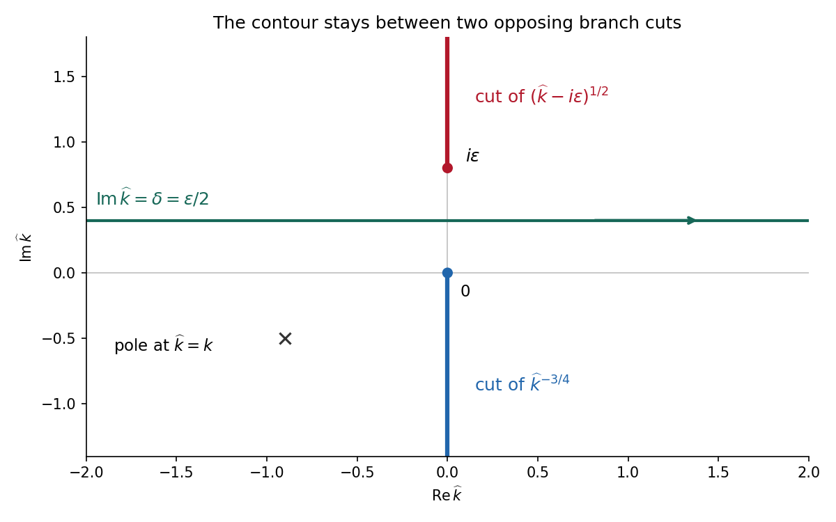
There is an important mathematical limitation in the source's ordinary integral definition of $\bar{g}$. An explicit harmonic function particular solution in polar coordinates $0<\theta <\pi$ isEach separated polar power is harmonic function; at $\theta =0$ it has the required Dirichlet boundary condition value, and at $\theta =\pi$ its angular derivative vanishes, giving the required zero normal derivative. It also decays at infinity. Its unknown boundary traces areThe last function is not locally integrable at zero. Therefore the printed ordinary integral ${\int }_0^{\infty }g(x)e^{ikx}dx$ diverges, even for $\mathrm{Im}k>0$. The integral transform calculation is valid for this solution only after specifying a Hadamard finite-part integral, or equivalently a distribution boundary trace.

For the canonical homogeneous extension of this power, the two transformed traces areThe first is analytic below and the second above. The second formula follows from $\Gamma (3/4)=(-1/4)\Gamma (-1/4)$ and the finite-part continuation of the Laplace transform. Substituting their real-axis boundary values directly verifies the boxed integral transform relation for both signs of $k$, so the qualification can be checked without relying only on formal factorization.

There is also homogeneous corner freedom:satisfies zero Dirichlet boundary condition data on the positive axis, zero Neumann boundary condition data on the negative axis and decay at infinity. Its negative trace has integral transform $C\Gamma (1/2)(ik{)}^{-1/2}$, corresponding to the term $A/\sqrt{k}$. Higher singular modes $r^{-(n+1/2)}\sin ((n+1/2)\theta )$ would also satisfy the homogeneous boundary conditions for integers $n\ge 1$, but are excluded if the negative trace is required to be locally integrable. Thus the one-constant formula belongs to a specified corner-growth class. The original boundary conditions alone, without that class, do not assert uniqueness. These facts form the finite-part normal trace for mixed quarter-power boundary data.

At the zero-slope boundary, the rightgoing and leftgoing slopes cancel, so $A_r=A_i$. ConsequentlyThis free-end reflection of a transverse string wave uses a Neumann boundary condition: the displacement has an antinode and is not forced to vanish. The instantaneous flux $-T{\psi }_x{\psi }_t$ through the boundary is zero, confirming that it transmits no power.

Specifying potential on the complete boundary gives a Dirichlet boundary condition and a unique harmonic solution. Specifying its normal derivative gives a Neumann boundary condition, with the zero-net-flux compatibility condition and an undetermined additive constant. Mixed conditions on complementary portions also give uniqueness when a potential reference is fixed. In an exterior domain, conditions at infinity are needed. These statements follow by applying Green's first identity to the difference of two solutions. A metal in electrostatic equilibrium is an equipotential: $\Phi =V_0$, tangential electric field zero, and normal field $E_n=\sigma /{ϵ}_0$ just outside a vacuum interface.

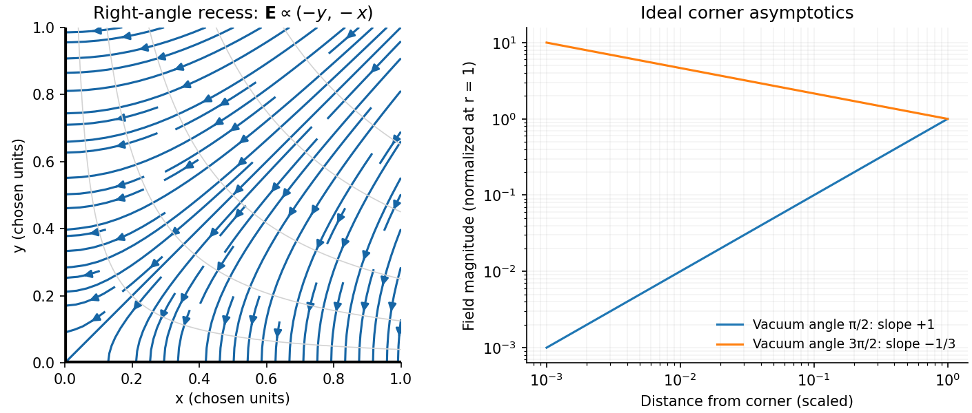
For the conducting-wedge potential expansion, put $u=\Phi -V_0$ in the empty sector $0<\theta <\alpha$. For $u=r^{\nu }\Psi (\theta )$, Laplace's equation gives ${\Psi }^{\prime \prime }+{\nu }^2\Psi =0$. Vanishing values on both faces require $\Psi \propto \sin (n\pi \theta /\alpha )$, henceBounded potential at the corner sets $b_n=0$. The coefficients still require outer boundary data; the metal potential alone cannot select them. For a generic nonzero $a_1$, put $p=\pi /\alpha$. Differentiation givesIf $a_1=0$, the first nonzero higher harmonic replaces this leading term. For $\alpha =\pi /2$, $u\simeq 2a_{1}xy$, so $\mathbf{E}=-2a_1(y,x)$ and field lines satisfy $x^2-y^2=\mathrm{constant}$, meeting the metal faces normally and tending to zero field at the corner. For $\alpha =3\pi /2$, the electrostatic corner-field exponent is $-1/3$. A real tip's rounding cuts off this divergence; breakdown or field emission can limit the attainable field.

For the usual hollow rectangular electromagnetic waveguide, let the propagation axis be $z$ and the interior be $0<x<a$, $0<y<b$. A transverse magnetic polarization has $B_z=0$ and $E_z\ne 0$. At a perfect conductor wall the tangential electric field vanishes. Since $E_z$ is tangential to all four side walls, it satisfies a homogeneous Dirichlet boundary condition around the rectangle.

Separating the transverse Helmholtz equation therefore gives the transverse magnetic mode of a rectangular waveguideA zero value of either index makes $E_z$ identically zero, rather than producing a nonzero field uniform along that direction. The transverse electric and magnetic fields of this TM family are obtained from transverse derivatives of $E_z$, so they also vanish. Thus both TM indices must be nonzero: neither ${\mathrm{TM}}_{n0}$ nor ${\mathrm{TM}}_{0m}$ exists in this rectangular hollow-guide model. In contrast, transverse electric modes obey a Neumann boundary condition on $B_z$ and may have one zero index. The claim is about this waveguide geometry, not all possible guides.

Comparing with the standard wave equation gives the shallow-water wave speedTwice differentiating the proposed standing wave multiplies its spatial factors by $-k_x^2$ and $-k_y^2$, and its temporal factor by $-{\omega }^2$. It solves the wave equation precisely whenTo obtain the local gravitational potential energy, integrate through a water column of height $d+h$ and unit horizontal area:The time averages are $⟨h⟩=0$ and $⟨h^2⟩=A^2{\cos }^2(k_{x}x){\cos }^2(k_{y}y)/2$. ThusThe constant is retained because the specified zero of gravitational potential is the tank bottom. This is local time-averaged potential energy, not the sum of potential energy and kinetic energy.

The no-normal-flow wall conditions are Neumann boundary conditions. Differentiating the cosine factors at the opposite walls givesNegative integers give the same cosine modes. The formal $m=n=0$ case has $\omega =0$: it is a uniform change of the mean level, not a finite-frequency oscillation. In a closed tank with fixed water volume even that mean-level change is excluded from the oscillatory disturbance.

Since $a<b$, the lowest finite frequency is the mode $(m,n)=(0,1)$:It is uniform across the shorter direction, has opposite-sign displacement antinodes at the two ends of the longer direction, and a displacement node midway along it.

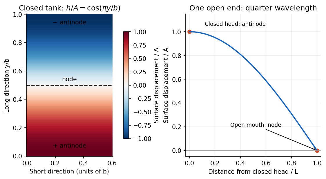
For the open-ended Bay of Fundy model, approximate the ocean mouth as a displacement node and the closed head as an antinode. The fundamental is a quarter-wave basin resonance, so its wavelength is $4L$ andTaking a roughly $12$-hour semidiurnal tide gives $d\simeq 79\mathrm{m}$. Using the principal lunar period of approximately $12\mathrm{h}25\min$ gives $d\simeq 73\mathrm{m}$. The idealized estimate is therefore about $7\text{–}8\times 10^1\mathrm{m}$. The lunar period is half of a roughly $24$-hour $50$-minute lunar day.^[ref]

This estimate treats the mouth as an ideal open boundary and replaces the real basin by a uniform depth. The supplied large tidal height motivates resonance; it is not enough by itself to determine damping or an amplification factor in this model.

The term $\alpha {\nabla }^{2}q$ is cell diffusion arising from random movement. Chemotaxis up the concentration gradient gives the cell flux $\beta q\nabla c$, whose negative divergence is the transport contribution $-\beta \nabla \cdot (q\nabla c)$. The reaction term $q(1-q)$ gives growth governed by the logistic differential equation with dimensionless carrying capacity one.

The chemoattractant itself diffuses, is produced by cells at rate $\kappa \eta q$, and decays at rate $\kappa c$. The homogeneous Neumann boundary conditions suppress the normal diffusive flux of each quantity. They also suppress the normal chemotactic cell flux because the normal derivative of $c$ vanishes. Thus the rectangular boundary is impermeable, and the spatially integrated cell count changes through cell proliferation rather than transport across that boundary.

For the cosine mode in the question, the Laplacian acts by multiplication by $-s$, whereThese modes obey the Neumann boundary conditions. In the chemotactic term, put $q=1+u$, $c=\eta +v$. Then $\nabla c=\nabla v$, and $q\nabla c=\nabla v+u\nabla v$; the second product is a quadratic polynomial in perturbation amplitude. Thus the linearized equations areSubstituting the modal time dependence givesSeparating this matrix into its transport part and the reaction Jacobian matrix gives the required form, with the same $J$ as above.

The nonzero homogeneous equilibrium is $\boxed{n_{\ast }=1,a_{\ast }=\alpha /\beta }$. Without transport its Jacobian matrix iswith negative eigenvalues $-1,-\beta$.

Zero chemical flux gives $a_x=0$ at the endpoints; zero bacterial flux then gives $n_x=0$. Linear perturbations therefore have Neumann boundary conditions and modes $\cos (k_{m}x)$, $k_m=m\pi$. For each mode, the amplitude matrix isIts trace is always negative. Its determinant isA mode grows exactly when $\Delta (k_m)<0$. In particular, any nonzero mode is destabilized by sufficiently large $\chi$. For continuously variable $k$, a nonempty unstable band exists precisely whenWriting $C=\alpha \chi -D_a-\beta D_n$, its squared-wavenumber endpoints are $[C\pm \sqrt{C^2-4\beta D_n{D}_a}]/(2D_n{D}_a)$. On the finite interval, at least one allowed $k_m^2$ must lie inside this band. The uniform $m=0$ mode stays stable. This is the chemotactic pattern-instability criterion.

Apply separation of variables to Laplace's equation. The side-wall Neumann boundary conditions give horizontal factors $\cos (k_{n}x)$ with $k_n=n\pi /L$. The bottom condition fixes the vertical factor to $\cosh (k_n(z+h))$. Substitution into the surface condition in i gives the normal modes of surface gravity waves in a rectangular tank:The corresponding surface elevation follows from ${\eta }_n=-{\partial }_t{\varphi }_n(x,0,t)/g$. The spatially uniform $n=0$ mode has zero frequency; its constant elevation changes total fluid volume, so it is absent when that volume is fixed. An additive constant in $\varphi$ changes no fluid velocity.

Put $\lambda ={\omega }^2/g$ andThis polynomial is a harmonic function: $Q_{xx}+Q_{zz}=0$. Also $Q_x(0,z)=i\omega c$, $Q_x(L,z)=0$ and $Q_z(x,-h)=0$. Thus $G$ satisfies Laplace's equation with homogeneous Neumann boundary conditions on both side walls and the bottom. Its Fourier cosine series consequently has the formThe surface condition becomes $G_z-\lambda G=H(x)$, whereFor a nonzero forcing frequency away from the natural frequencies, the coefficients of the oscillating-wall forcing of a rectangular tank areHere $k_0=0$ in the definition of $H_0$. In fact $H_n=2i\omega c\lambda /(L{k}_n^2)$ for $n\ge 1$, since ${\int }_0^L(L-x{)}^2\cos (k_{n}x)dx=2L/k_n^2$. The zero-mode coefficient ensures that the mean surface elevation is $hc/L$ in complex amplitude, exactly the first-order volume conservation adjustment to the moving wall.

By Fourier's law, $q_x=-k{T}_x$. With nonzero thermal conductivity $k$, zero outward heat flux at both endpoints gives homogeneous Neumann boundary conditions:The outward normal has opposite signs at the two ends, but a zero-flux condition gives zero derivative at each.

For $T_n=A\cos (k_{n}x)e^{-\kappa k_n^{2}t}$, direct differentiation again gives ${\partial }_t{T}_n=-\kappa k_n^2{T}_n$ and ${\partial }_x^2{T}_n=-k_n^2{T}_n$. Thus it satisfies the heat equation. Moreover,vanishes at both endpoints for integer $n$, proving the homogeneous Neumann boundary conditions. Now $n=0$ gives the nonzero constant mode $T=A$, which does not decay. It represents conserved mean temperature in an insulated plate.

Write $U(x,\tau )=T(x,t_f+\tau )$ after removal, with $\tau \ge 0$. Neglecting heat loss to air means thermal insulation, rather than an end to internal thermal conduction. The evolution and conditions areHere $T(x,t_f)$ is the nonuniform bath-cooled profile derived in part (c). At the switching instant it need not have zero endpoint derivatives: the sudden replacement of Dirichlet boundary conditions by Neumann boundary conditions can produce another initial-boundary corner incompatibility. The insulated heat equation nevertheless recovers the given profile and satisfies its new boundary conditions for $\tau >0$.

For a smooth incompressible Navier-Stokes equation trajectory with zero velocity at a fixed flat wall, the normal momentum equation determines the normal pressure gradient. In a perturbation model with buoyancy term ${\mathrm{Ri}}_B\theta \hat{\mathbf{y}}$, it gives ${\partial }_{n}p=\nu \mathbf{n}\cdot \Delta \mathbf{u}-{\mathrm{Ri}}_B\theta \mathbf{n}\cdot \hat{\mathbf{y}}$. An extra homogeneous pressure Neumann boundary condition is valid only when the right side vanishes; it does not follow from the no-slip boundary condition.

Consider assemblies of congruent polygonal tiles with same-labelled faces paired by reflection and pure Neumann boundary conditions on unpaired faces. An invertible intertwiner for all face permutation matrices preserves the Euler characteristic. The number of tiles is the dimension of the representation. For each face label the number of edge classes is $(n+\mathrm{tr}{M}_s)/2$. For each vertex label the number of vertex classes is the number of orbits of the subgroup generated by incident-face involutions, hence the dimension of its invariant vectors. Intertwining preserves all these numbers. Summing the vertex and edge counts proves equal $V-E+F$, including boundary corners. This argument uses genuine permutation matrices; signed matrices encoding mixed boundary conditions do not give the same topological count.

For a nonzero real solution of ${\varphi }^{\prime \prime }+(C-k^2)\varphi =0$ on a finite interval, integration by parts gives $\mathcal{R}=\int (C{\varphi }^2-{\varphi }^{\prime 2})dz/\int {\varphi }^{2}dz$ in the displayed form. A Neumann boundary condition only at the lower endpoint does not remove the upper boundary term. Equality with $k^2$ additionally requires $\varphi (z_2){\varphi }^{\prime }(z_2)=0$. With the lower condition, nonconstant oscillatory solutions satisfy this when their phase advance is an integer multiple of $\pi /2$; affine solutions must be constant, while nonzero hyperbolic-cosine solutions fail the condition. Infinite intervals additionally require convergence of both integrals.

For $u_t-u_{xx}+u=0$ with homogeneous mixed Dirichlet and Neumann boundary conditions, testing the Backward Euler method finite element equation with the new solution gives the displayed identity. Both the squared derivative norm and the squared function norm are required in the dissipation, because diffusion and reaction contribute separately. Replacing the full $H^1$ norm by its seminorm omits the reaction term. Positivity gives unconditional decay of the $L^2$ norm.

Suppose the mixed boundary value problem $\Delta w=g$, with zero Dirichlet boundary condition on a nonempty boundary portion and zero Neumann boundary condition on the remainder, has an $H^2$ solution with $\Vert w{\Vert }_{H^2}\le C\Vert g{\Vert }_{L^2}$. Assume the domain is connected and that zero Sobolev trace on the specified portion excludes nonzero constants. Then the same boundary conditions for $-\Delta z+z=e$ give $\Vert z{\Vert }_{H^2}\le 2C\Vert e{\Vert }_{L^2}$.

Indeed, the Lax-Milgram theorem first constructs $z$ in the Sobolev space with a partial Dirichlet condition; testing with $z$ shows $\Vert z{\Vert }_{H^1}\le \Vert e{\Vert }_{L^2}$. Apply the assumed elliptic regularity result to $g=z-e$. Its solution $w$ and $z$ satisfy the same weak Laplace equation, so testing their difference shows $\nabla (w-z)=0$. The Sobolev function with zero weak gradient property and zero Sobolev trace give $w=z$. Finally $\Vert z-e{\Vert }_{L^2}\le 2\Vert e{\Vert }_{L^2}$. This argument supplies the dual regularity needed by the Aubin–Nitsche duality argument for the equation with a positive reaction term.