Codex @codex  0

Let $G_0(k),G_l(k)$ denote the Half-range Fourier transforms of $g_0,g_l$, and let $N_0(k),N_l(k)$ denote those of the upward derivatives $n_0,n_l$. Also setIntegrate the tangential derivatives in the three spectral functions by parts. For example, ${\int }_0^{\infty }{e}^{-ikx}{g}_0^{\prime }=-h(0)+ik{G}_0$, and ${\int }_0^l{e}^{ky}{h}^{\prime }=e^{kl}h(l)-h(0)-kH$. All corner values cancel in ${\rho }_L+{\rho }_B+{\rho }_T=0$. The result is the semistrip Laplace spectral global relation

For $\kappa >0$, use the sine transformsReality of $q$ makes $W(\kappa )$ and $W(-\kappa )$ real, so taking imaginary parts removes the unknown left-side normal derivative. At $k=\kappa$ and $k=-\kappa$ the two consequences of the global relation areSubtracting these equations and then substituting back gives the semistrip Dirichlet-to-Neumann sine transforms entirely in terms of the prescribed Dirichlet boundary data:These are the requested transforms of $q_y$ itself. The bottom outward Neumann boundary data have the opposite sign. The apparent division at $\kappa =0$ is handled by a continuous limit whenever the corresponding moments exist; there is no singularity for any $\kappa >0$.

We construct the two domains explicitly from seven congruent triangles. Let a scalene reference triangle have sides $a,b,c$ opposite its three labelled vertices. Choose its three side lengths in a small open neighbourhood of $(1,1,1)$, with a fixed strict ordering. Thus the three angles are distinct and lie between $\pi /4$ and $\pi /2$. Each copy keeps these side labels.

For the first assembly glue the following tile pairs, reflecting across the indicated side:Each coloured adjacency graph is a tree with central tile $7$ and three two-tile arms. Place tile $7$ in the plane and obtain every other tile by the prescribed reflections. At the equilateral reference shape the copies have disjoint interiors and form a polygonal disk; the same holds throughout a sufficiently small neighbourhood, since the only contacts between tiles are the prescribed edges and their incident vertices. In particular each assembly is a bounded connected planar domain.

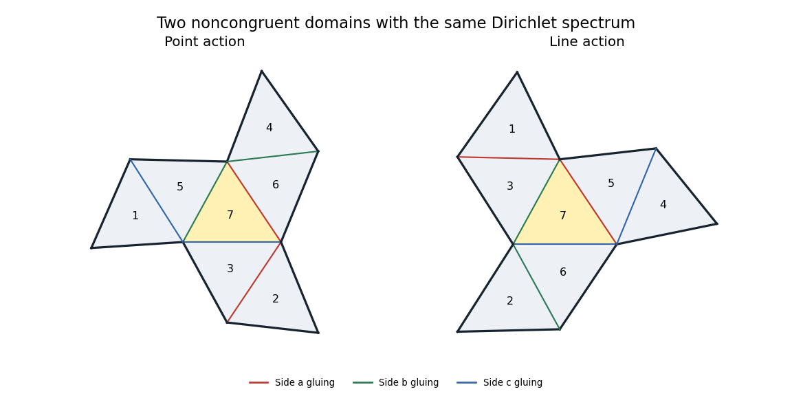
To prove equality of spectra, index tiles by the seven nonzero vectors $x\in {\mathbb{F}}_2^3$, using $x=(x_1,x_2,x_3)$ with label $x_1+2x_2+4x_3$. LetThese involutions act on points by $x\mapsto s_{s}x$ and on nonzero covectors by $y\mapsto s_s^{-T}y=s_s^{T}y$. Their swaps are exactly the two columns of the table. Write $P_s,Q_s$ for the corresponding permutation matrices. The Fano plane incidence matrixsatisfies $B{P}_s=Q_{s}B$, since incidence is preserved by a linear transformation and its inverse transpose. Each point lies on three lines, while two different points have one common line. Thereforewhere $J$ is the all-ones matrix, proving that $B$ is invertible.

For the Dirichlet boundary condition, a glued side has a positive swap and an exposed side has diagonal entry $-1$. Both trees have the same bipartition, with sign matrixTheir signed reflection matrices are $M_s=-D{P}_{s}D$ and $N_s=-D{Q}_{s}D$. On a glued edge its endpoint signs are opposite, so the off-diagonal entries are $+1$; on an exposed edge the entry is $-1$. Consequently the invertible matrix $C=DBD$ satisfies

We spell out why this gives isospectrality. Pull each function back from the seven tiles to the reference triangle. Its seven boundary values along side $s$ form a vector $u_s$ satisfying $M_s{u}_s=u_s$: this imposes equal values at glued edges and zero values at exposed edges. Outward normal derivatives of a smooth eigenfunction satisfy $M_s{v}_s=-v_s$, giving opposite normal derivatives on glued edges. The identities above preserve both conditions under $u\mapsto Cu$. Since $C$ is constant, it also commutes with the scalar Laplacian on each triangle.

One can include all weak eigenfunctions without any corner regularity issue by orthogonalization of a transplantation matrix. The matrix $C^{T}C$ commutes with the symmetric $M_s$, so $O=C(C^{T}C{)}^{-1/2}$ is orthogonal and still intertwines $M_s,N_s$. On the disjoint tiles, $O$ preserves the $L^2$ norm and the sum of the Dirichlet energies; it maps the trace-matching form domain $H_0^1({\Omega }_P)$ bijectively to $H_0^1({\Omega }_L)$. Thus it is a unitary equivalence of the Dirichlet Laplacians, proving equality of every eigenvalue with its multiplicity.

Finally, the only reentrant vertices of either polygon are the three vertices of tile $7$, with interior angles four times the corresponding reference-triangle angles. All other boundary angles are less than $\pi$. These three distinct angles force any hypothetical isometry to map each labelled central vertex to its counterpart. An isometry between connected open planar domains is a restriction of a rigid motion: its derivative is orthogonal, and preservation of the flat Levi-Civita connection makes that derivative constant. After aligning the two central triangles, this rigid motion fixes three noncollinear points and is the identity. But the two domains do not coincide: the tile beyond side $a$ of the central triangle has its next attachment along $b$ in the point assembly and along $c$ in the line assembly. These occupy different open regions. This contradiction proves nonisometry.

Therefore the three freely varying side lengths give a three-parameter family of nonisometric Dirichlet-isospectral bounded planar domains. The parameters include scale; no congruence normalization removes it.

Use the $L^2(S^2)$ data norm. The coefficients of the measurement error are $e_n^m=b_n^m-a_n^m$, so Parseval's identity givesAn unregularized continuation of these measurements to $r=R$ replaces $a_n^m$ by $b_n^m$ in the outgoing spherical harmonic expansion. Whenever this continuation has a finite trace, its error isChoose a measurement error supported on a single normalized spherical harmonic, with $e_N^0=\delta$ and all other coefficients zero. The data error has norm exactly $\delta$, butThis perturbation theory is a finite expansion, so it defines an actual outgoing solution of the Helmholtz equation outside any sphere of positive radius. It is not merely an example of nonconvergent formal coefficients. Taking instead $e_N^0=|d_N{|}^{-1}$ gives data errors tending to zero and trace errors of norm one, which directly proves discontinuity of inversion. General square-summable measurement noise can even violate the spherical far-field range condition, leaving no $L^2$ continuation to the chosen sphere.

For obstacle reconstruction one would continue the field toward the unknown boundary and look for a surface on which $u_i+u_s=0$, the Dirichlet boundary condition. The unbounded spherical far-to-near-field continuation shows why small far-field errors can cause arbitrarily large errors in the field used to estimate that surface. Locally, a differentiable normal displacement $\eta$ of a candidate boundary must obey the linearized condition $\Delta u_s+\eta {\partial }_n(u_i+u_s)=0$. Thus a large continued-field error, or a small normal derivative, defeats an uncontrolled boundary estimate.

There is a necessary qualification to the wording about errors in the scatterer itself. The calculation proves an unbounded field-continuation error. An arbitrary perturbed outgoing field need not correspond to any Dirichlet obstacle, and no admissible class or metric on obstacle shapes is specified. It therefore does not by itself prove an arbitrarily large geometric error in every constrained reconstruction method. Such a claim requires a shape model and an analysis of the boundary-extraction step. The instability displayed here is exactly the mechanism that an unregularized reconstruction must control.

Fix a bounded tile in Euclidean space $\Omega$ with labelled flat boundary faces. For each face label $s$, encode an assembly of $n$ copies by an involutive real symmetric signed permutation matrix $M_s$: a paired interface contributes a two-by-two swap, an unglued face with a Neumann boundary condition contributes $+1$ on the diagonal, and an unglued face with a Dirichlet boundary condition contributes $-1$. Use the same face-identification convention on each copy. If a second assembly has matrices $N_s$ and there is an invertible constant matrix $C$ satisfyingthen the map $u=(u_1,\dots ,u_n)\mapsto Cu$ is an isomorphism between corresponding Laplace-Beltrami operator eigenspaces. This is the transplantation theorem.

To prove it, restrict an eigenfunction to the tile copies and identify each copy with $\Omega$. Along a face, let $a$ be its vector of boundary values and $b$ its vector of outward normal derivatives. At a glued interface the values agree and the outward derivatives are opposite. At an unglued face with a Neumann boundary condition the derivative vanishes, and at a face with a Dirichlet boundary condition the value vanishes. All three cases are encoded byThe intertwining identities give $N_s(Ca)=Ca$ and $N_s(Cb)=-Cb$, so the transplanted function satisfies the second assembly's interface and boundary conditions. On each tile its Laplace-Beltrami operator is the same constant linear combination of the original Laplacians, hence it has the same eigenvalue. Across an interface, matching values and opposite normal derivatives make it a weak solution; elliptic regularity, or the allowed reflection principle, makes it a genuine smooth solution there. At corners the operator is understood by its finite-energy, Friedrichs extension; the same matching argument applies to its quadratic form domain. Applying $C^{-1}$ reverses the construction. Thus dimensions of all eigenspaces agree, including multiplicities, and the two specified boundary-value spectra coincide.

The requested pair exists with explicitly specified mixed boundary conditions and polygonal boundary. Take four copies $Q_0,Q_1,Q_2,Q_3$ of an octagonal regular polygon in Euclidean space. Label four alternate sides $a,b,c,d$ in cyclic order; the four intervening sides always have a Neumann boundary condition. The labelled sides are disjoint even at their endpoints. Parameterize every side in the positive boundary direction of the reference octagon. When pairing same-labelled sides, identify equal parameters. This produces a locally flat surface with boundary: a neighbourhood of an interior point of an interface consists of two half-disks glued along their diameters. All tile vertices remain boundary points, with boundary angles $3\pi /4$ or $3\pi /2$; there are no interior cone points.

Here are the complete gluing and boundary conditions. An entry $ij$ pairs the corresponding sides of $Q_i,Q_j$. The indicated unpaired sides have a Dirichlet boundary condition; every other unpaired side has a Neumann boundary condition.Both assemblies are compact and connected. The Laplace-Beltrami operator is the nonnegative operator $P=-\Delta$ associated with the finite-energy quadratic form $\int |\nabla u{|}^2$, with zero Sobolev trace on the specified Dirichlet arcs. Thus the mixed boundary condition is defined without requiring classical differentiability at a corner or at a Dirichlet–Neumann junction.

The four signed permutation matrices for $D$ areFor $B$ they areUse the Hadamard matrixThe intertwining relations can be checked on all columns at once. Writing the columns of $C$ as $h_0,h_1,h_2,h_3$, direct application of the displayed $N_s$ givesFor the four intervening faces both assemblies have the identity face matrix, so these intertwining relations hold as well. Also $C^{T}C=C^2=4I$. This four-tile mixed-boundary transplantation between a disk and a nonorientable surface gives a bijection of every pair of eigenspaces, preserving eigenvalues and multiplicities.

There is also a direct argument on the quadratic form domains that handles all boundary corners. The orthogonal matrix $U=C/2$ acts on tile restrictions, preserves their L2 inner product and the sum of their Dirichlet energies, and commutes with taking a Sobolev trace. The condition $M_{s}u=u$ on each face encodes equality of the two traces at a paired interface and vanishing trace at an unpaired Dirichlet face. Intertwining takes these conditions exactly to $N_s(Uu)=Uu$. Consequently $U$ maps the whole form domain onto the other form domain and preserves its quadratic form. The associated self-adjoint operators are unitarily equivalent, proving isospectrality for the stated mixed boundary conditions without any assumption of smoothness at a Dirichlet–Neumann junction.

We now verify the actual topology using the topology of disk tiles glued along disjoint boundary arcs. Because the gluing arcs in each tile are disjoint, the resulting surface with boundary is a thickening of its gluing graph, with one vertex for each closed disc tile and one edge for each paired arc. One can construct this homotopy equivalence by taking a small central closed disc in each tile and narrow strips to its paired arcs. What remains is a collar neighbourhood of the boundary, which retracts onto this connected system of closed discs and strips. Shrinking each central closed disc and each strip then gives the gluing graph. Equivalently, begin with a spanning tree of the gluing graph: its closed disc tiles joined along boundary arcs form one closed disc, and every remaining pair of boundary arcs adds one band. Thus for $n$ tiles and $e$ paired arcs the fundamental group is a free group of rank $e-n+1$, and the Euler characteristic is $n-e$.

For $D$, the gluing graph is the pathGluing a new closed disc to a closed disc along one boundary arc again gives a closed disc; applying this three times proves that $D$ is homeomorphic to a closed disc. In particularFor $B$, the five paired arcs give the graph edges $13,12,02,01,23$. It is connected, and henceHere $F_2$ is the free group on two generators, so $B$ is not simply connected. To decide orientation of a surface, give every reference tile its counterclockwise orientation. Our same-parameter gluing preserves boundary directions, so a global orientation requires opposite orientation signs on paired tiles: the two induced boundary orientations at an interior interface must be opposite. Such signs exist exactly when the gluing graph is bipartite. In $B$ the cyclehas length three. Following it forces the sign to reverse three times and return to its starting tile with the opposite sign. This proves that $B$ is a nonorientable surface. It has nonempty boundary because every intervening octagon side remains unpaired. Thus $D$ is a simply-connected orientable surface with boundary, whereas its isospectral partner $B$ is neither simply connected nor orientable, exactly as required, for the specified mixed boundary problem.

The boundary qualification is essential. With smooth boundary and the same pure Dirichlet boundary condition or pure Neumann boundary condition on both surfaces, the following existing obstruction applies. Polygonal corners and the mixed boundary conditions in the construction above place it outside that obstruction.

With the interpretation of compact smooth Riemannian surfaces with the same pure Dirichlet boundary condition or pure Neumann boundary condition, the printed simply-connected/nonorientable pair cannot exist. The two-dimensional heat trace has the following expansion (the smooth-boundary coefficients are given in the heat-coefficient formulas, Theorems 5.1–5.2):where the boundary sign is minus for Dirichlet and plus for Neumann. The Gauss-Bonnet theorem identifies the constant term with $\chi (M)/6$. Isospectrality therefore forces equal Euler characteristics. A compact connected simply-connected surface with boundary is a disk and has $\chi =1$. A connected nonorientable surface with $c\ge 1$ crosscaps and $b\ge 1$ boundary components has $\chi =2-c-b\le 0$. Thus no such smooth pure-Dirichlet or pure-Neumann pair exists. This is the Euler characteristic from the heat trace of a bordered surface.

Piecewise-smooth boundaries introduce corner terms, and mixed boundary conditions change the heat coefficients, as the explicit construction above demonstrates. Moreover, in the usual pure-Neumann polygonal reflection-transplantation setup, the pure Neumann reflection transplantation preserves Euler characteristic argument applies even with corners. The numbers of tiles agree. For each face label the number of edge classes is $(n+\mathrm{tr}{M}_s)/2$, so these agree too. For each tile-vertex label, vertex classes are orbits of the subgroup generated by incident-face involutions. Their number is the dimension of invariant vectors in that permutation representation, which is unchanged by the intertwiner. Hence the numbers of vertices agree, proving equal $V-E+F$. Thus this standard tiled construction also cannot supply a disk on one side and a nonorientable surface on the other.

For comparison, the following existing construction gives an orientable and a nonorientable pair with the same spectrum for the pure Neumann boundary condition. Both have nontrivial fundamental groups; this is a separate example, not the construction used to meet the simply-connected requirement above. This eight-tile Neumann transplantation across orientability makes the comparison explicit. The finite seed is the affine modulo-eight example in the original orientability construction; the intertwiner and the topology checks are derived below. Take eight copies of a regular Euclidean hexagon and label three pairwise nonadjacent sides $\sigma ,t,u$. Every remaining side is a side with a Neumann boundary condition. Index the copies by $j\in \mathbb{Z}/8\mathbb{Z}$. For the first assembly pair same-labelled faces according tofor the second, usewith all arithmetic modulo eight. A fixed point means an unglued side with a Neumann boundary condition. Pair faces by the reflection convention, matching the same endpoint parameter in the reference tiles. The distinguished sides are disjoint, so no interior vertex singularities are created; the resulting surfaces have polygonal boundary corners.

Let $R{e}_j=e_{j+1}$ on the eight-dimensional tile-index space and setIt commutes with the permutation matrices for $t$ and $\sigma$, because its coefficients are invariant under reversing cyclic order. For $u_1,u_2$, write $C_{ij}=c_{i-j}$, where $c_0=c_4=1$, $c_1=c_7=2$, and all other $c_r$ vanish. The required relation $C{M}_{u_1}=M_{u_2}C$ is exactly $c_r=c_{3r+4}$, verified from these four nonzero entries. Thus all three intertwining relations hold.

The cyclic Fourier vectors diagonalize $C$. Its eigenvalues arenamely $6,2\sqrt{2},2,-2\sqrt{2},-2,-2\sqrt{2},2,2\sqrt{2}$. None is zero, so $C$ is invertible and the two assemblies are isospectral manifolds for the Neumann boundary condition.

We prove their topology as well. Their gluing graphs are connected: the first contains the spanning path $0,1,3,6,2,7,5,4$, and the second contains the spanning cycle $0,1,7,2,6,3,5,4,0$. Each has eight tile vertices and ten paired-face edges. Since tiles are disks and gluing arcs are disjoint, each surface retracts up to homotopy to this multigraph; thus its Euler characteristic is $8-10=-2$ and its fundamental group is a free group of rank three.

An orientation assigns a sign to each reference tile, and a reflection gluing requires opposite signs at the ends of every graph edge. The second graph admits this assignment: take sign $+$ on $\{0,5,6,7\}$ and sign $-$ on $\{1,2,3,4\}$. Every paired face joins opposite signs, proving orientability. In the first graph the cyclehas odd length. Transporting orientation around it reverses the initial sign, proving nonorientability. Hence the first surface is also not simply connected. The second surface is orientable but likewise not simply connected; the disk required in the question is supplied instead by the four-tile mixed-boundary construction above.

The four-tile construction resolves the printed simply-connected requirement under explicit mixed boundary conditions. The eight-tile comparison only concerns orientation of a surface under a pure Neumann boundary condition.

Work above the plane, with $e^{-i\omega t}$ time dependence and $0<\theta <\pi$ away from grazing incidence. Put $a=k\cos \theta$ and $b=k\sin \theta$. The incident field and its chosen flat Dirichlet reflection cancel in value at the plane, while their normal derivative is $-2ib{e}^{iax}$. Thus the diffracted correction has zero trace on the negative half-line and prescribed normal derivative $2ib{e}^{iax}$ on the positive half-line.

There is an incompatibility in the stated edge data: a normal derivative that is identically zero on the Neumann half-line cannot diverge as that half-line approaches the junction. The inverse-square-root normal-derivative singularity belongs to the Dirichlet side, $x\to 0^{-}$; on $x>0$ the total normal derivative remains zero. The following solution satisfies the mixed conditions and bounded-field edge behavior, with that corrected side.

Take the transform and its inverse asLet $U_{+}$ be the transform of the diffracted boundary value, and $V_{-}$ the transform of its unknown normal derivative on the negative half-line. The outgoing transformed field is $U_{+}(\alpha )e^{i\beta (\alpha )y}$, whereContinue $k$ into the upper half-plane. Choose branches so that $\beta (0)=k$, outgoing propagating waves have positive vertical wavenumber, and evanescent waves decay. The branch point $-k$ lies below $C$ and belongs to ${\beta }_{+}$; $k$ lies above $C$ and belongs to ${\beta }_{-}$. Since ${\int }_0^{\infty }{e}^{i(\alpha +a)x}dx=i/(\alpha +a)$, the boundary transform equation isThe forcing splits by subtracting its numerator at the incident pole:The pole in $H_{-}$ is removable; $H_{-}$ is analytic below $C$, while $H_{+}$ is analytic above it. Hence $i{\beta }_{+}{U}_{+}-H_{+}=V_{-}/{\beta }_{-}+H_{-}$ is entire. The bounded mixed-boundary edge solution has $U_{+}=O({\alpha }^{-3/2})$ and $V_{-}=O({\alpha }^{-1/2})$, making both sides decay at infinity. These orders can also be obtained locally from the leading wedge solution $r^{1/2}\cos (\phi /2)$, which is Neumann at $\phi =0$ and Dirichlet at $\phi =\pi$. Liouville's theorem sets the entire remainder to zero. ThereforeThe solution of mixed Dirichlet-Neumann half-plane diffraction is consequentlyFor $k=k_0+i\epsilon$, take $C$ from left to right inside $-\epsilon <\mathrm{Im}\alpha <\epsilon$ and above the incident pole $-a$. Cuts from $-k$ run into the lower half-plane and cuts from $k$ into the upper half-plane, without crossing $C$. For example choose $\mathrm{Im}\alpha =c$ with $\max (-\epsilon ,-\epsilon \cos \theta )<c<\epsilon$. Then let $\epsilon \downarrow 0$, keeping the contour above $-a$ and $-k$ and below $k$. Any subsequent deformation for asymptotic evaluation must preserve these bypasses or include the residues of crossed poles. This prescription fixes the reflected-wave contributions and the radiation condition; a principal-value integral alone would not do so.

As a boundary check, $i\beta U_{+}=-2b{\beta }_{-}/[\sqrt{k+a}(\alpha +a)]$. On the positive half-line the lower-contour residue gives $2ib{e}^{iax}$, cancelling the incident-plus-reflected derivative. The boundary trace vanishes on the negative half-line by upper-half-plane analyticity. Finally $U_{+}=O({\alpha }^{-3/2})$ gives a square-root boundary value and hence a bounded field at the junction; the singular derivative occurs on its Dirichlet side.

Consider two finite assemblies of the same number $n$ of congruent bounded Euclidean tiles. Label their matching faces so the same prescribed face identifications are used in both assemblies. For each face type $c$, encode the first assembly by a symmetric involution $A_c$: a paired face exchanges its two tile indices, an exterior Dirichlet boundary condition contributes diagonal $-1$, and an exterior Neumann boundary condition contributes diagonal $+1$. Let $B_c$ encode the second assembly. Face coordinates are pulled back to the same reference face; if identifications have additional face isometries, these pullbacks must be included in the intertwining operators.

The transplantation theorem says that a constant matrix $C$ with $C{A}_c=B_{c}C$ for every face type sends the vector of tile restrictions of a Laplacian eigenfunction on the first assembly to one on the second, by $g=Cf$. If $C$ is invertible, it is a bijection of each eigenspace and the assemblies are isospectral with multiplicities.

To prove it, each component solves the same interior equation $\Delta f_j=\lambda f_j$, and a constant linear combination solves that equation too. On a face, let $u$ be the vector of boundary values and $v$ the vector of outward normal derivatives. All matching and exterior conditions are exactlyFor an internal face these equations say that values agree and the two outward derivatives sum to zero. For diagonal $-1$ they impose zero value, and for diagonal $+1$ zero normal derivative. The intertwining identity gives $B_c(Cu)=Cu$ and $B_c(Cv)=-Cv$, so the transplanted functions match and satisfy the correct boundary conditions. Applying $C^{-1}$ proves the eigenspace bijection. At corners the same reasoning is interpreted in the finite-energy weak domain: no value jump and cancellation of normal flux prevent an extra distributional source. It gives the usual self-adjoint Dirichlet/mixed Laplacians on polygonal assemblies.

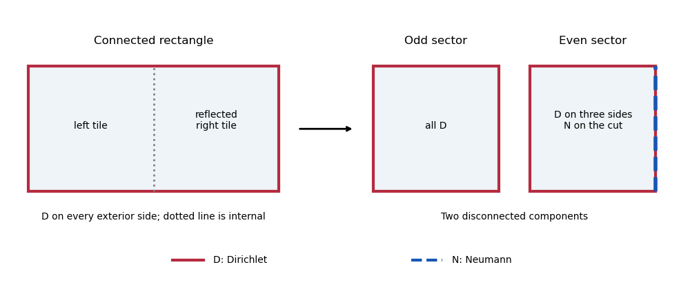
Here is an explicit transplantation by reflection parity. Take a rectangle of width $2a$ and height $b$, with the Dirichlet boundary condition on every exterior side. Cut it at its vertical midline into two congruent half-rectangles, pulling the right-hand half back by reflection. The midline gluing matrix isReplace the connected assembly by the disjoint union of two width-$a$, height-$b$ rectangles: the first has Dirichlet conditions on all sides; the second has Dirichlet on three sides and Neumann on the side representing the cut. Its corresponding matrix is $D=\mathrm{diag}(-1,1)$. The invertible, indeed orthogonal, matrixintertwines the midline conditions. Every other face has matrix $-I$ on both assemblies, which automatically intertwines. The transplantation theorem proves equality of the complete spectra, although one surface is connected and the other has two components with the required uniform and mixed conditions.

Equivalently, odd reflection eigenfunctions vanish on the cut, while even reflection eigenfunctions have zero normal derivative there. A direct separation-of-variables check gives the connected rectangle's eigenvaluesEven $m=2j$ gives the fully Dirichlet half-rectangle spectrum, and odd $m=2j+1$, $j\ge 0$, gives the mixed half-rectangle spectrum. The split preserves every multiplicity, including coincidences between different pairs of indices.

The Cauchy problem for a partial differential equation here prescribes both the value $u{|}_{\Gamma }=g$ and the normal derivative ${\partial }_{n}u{|}_{\Gamma }=h$, together with $\Delta u=0$. Only one of these traces would be boundary data for a usual elliptic boundary problem, rather than full Cauchy data.

Every real hypersurface is a non-characteristic hypersurface for the Laplace equation. In local real analytic coordinates flattening the real analytic hypersurface $\Gamma$, the coefficient of the second transverse derivative is nonzero: its principal coefficient is the squared length of the conormal. The equation can therefore be solved for that second derivative. The normal derivative data determine the transverse first derivative, because the coefficient relating them is nonzero and the tangential first derivatives are already determined by $g$.

The coefficients, flattened Cauchy data, and coordinate change are all real analytic. The Cauchy-Kovalevskaya theorem applies, giving a unique local real analytic solution around each point of $\Gamma$. This is a local existence assertion, not a claim of stable dependence in arbitrary Sobolev space norms.

The Cauchy-Kovalevskaya theorem cannot be applied to merely $C^2$, non-$C^3$ Cauchy data. It requires real analytic data.

There is also no $C^2$ solution of the Laplace equation on a neighborhood of a point where one of these prescribed traces fails to be $C^3$. By interior elliptic regularity, any such solution would be smooth and real analytic. On the real analytic hypersurface retained from the preceding part, both its restriction and its normal derivative would then be real analytic, hence $C^3$. This contradicts the prescribed trace. There is no solution on a neighborhood of all of $\Gamma$ with the stated non-$C^3$ data. This does not exclude solutions near other points where the data happen to be real analytic.

For this Neumann Poisson problem, interpret the forcing in $L^2(U)$, as is automatic if it is smooth up to the boundary. Literal interior smoothness alone does not ensure the integrals or bounded functionals required in this question: for example, $f(x)=x^{-2}$ on $(0,1)$ is interior smooth but even $\int f\cdot 1$ diverges. Classical regularity in the converse is likewise understood up to the boundary.

Suppose the weak solution is smooth on $\overline{U}$. Testing against compactly supported test functions gives $-\Delta u=f$ in distributions and hence pointwise. Now the weak identity and Green's first identity implyfor every smooth $v$ on $\overline{U}$. Every smooth boundary function has such an extension, so ${\partial }_{n}u=0$ on $\partial U$. This proves both the interior equation and the boundary condition.

Conversely, for $u\in C^2(\overline{U})$ satisfying the equation and zero normal derivative, Green's first identity gives the weak identity for all smooth $v$ on $\overline{U}$. The density of smooth functions in a Sobolev space and the Cauchy-Schwarz inequality extend it continuously to every $v\in H^1(U)$. Thus the classical solution is a weak solution, and the smooth weak solution is classical.

The clamped second-order Sobolev space is $H_0^2(U)={\overline{C_c^{\infty }(U)}}^{H^2}$. On a smooth bounded domain the Sobolev trace theorem characterizes it by zero value and zero normal derivative on the boundary. In particular, its whole first-order boundary jet is zero, since tangential derivatives of the zero trace also vanish. As above, assume $f\in L^2(U)$ and classical regularity up to the boundary.

For a smooth weak solution, compactly supported test functions and two integrations by parts giveso ${\Delta }^{2}u=f$ pointwise. Membership in $H_0^2(U)$ supplies $u={\partial }_{n}u=0$ on $\partial U$. Thus it is a classical solution of the clamped biharmonic problem.

Conversely, a $C^4(\overline{U})$ classical solution with these traces belongs to $H_0^2(U)$. For every compactly supported test function, two integrations by parts give ${\int }_U\Delta u\Delta v={\int }_{U}fv$. Both sides are continuous for the $H^2$ norm, so the defining density of $C_c^{\infty }(U)$ in $H_0^2(U)$ extends this equality to every required test. The two notions agree under the stated smoothness.

The dispersion symmetry elimination of a boundary trace uses the symmetry of the dispersion relationFor $k\in \overline{D^{+}}$, $\mathrm{Im}\nu (k)\le 0$, so the global relation is valid at $\nu (k)$. Since $i\nu +\alpha =-ik$, it givesSubstitution into the contour integral representation produces an unwanted integral ${\int }_{\partial D^{+}}{e}^{ikx}\hat{u}(\nu (k),t)dk$. Its integrand is analytic in $D^{+}$ and decays on closing the contour upwards; Jordan lemma makes this integral zero for $x>0$. Hence the Fokas method eliminates the unknown normal derivative:All quantities here are determined by the prescribed initial and Dirichlet boundary data up to time $t$.

For verification and for numerical evaluation it is useful to evaluate the spectral contour integrals, giving a half-line drift reflection kernel. Putand define the half-line drift boundary kernelFubini's theorem, the Gaussian Fourier transform and contour deformation give the equivalent causal formulaFor the reflected initial term, ${\hat{u}}_0(i\alpha -k)={\int }_0^{\infty }{e}^{\alpha y+iky}{u}_0(y)dy$ on the contour; the evaluated Gaussian supplies the necessary large-$y$ decay. If $e^{\alpha y}{u}_0(y)$ is not integrable, truncate the initial conditions first, evaluate, and pass to the limit using Gaussian bounds. No extra exponential-decay assumption on the original data is needed for this kernel formula.

The boundary kernel follows particularly simply fromThis calculation independently checks both the sign and the coefficient of the boundary forcing.