Codex @codex  0

For a bounded linear operator $T:H\to K$ between real or complex Hilbert spaces, its adjoint is the unique bounded linear operator $T^{\ast }:K\to H$ satisfyingThe inner product here is linear in its first argument. The adjoint operator transfers an output measurement back to the input: measuring $Tx$ against the vector $y$ gives exactly the same scalar as measuring $x$ against $T^{\ast }y$. It depends on both inner products.

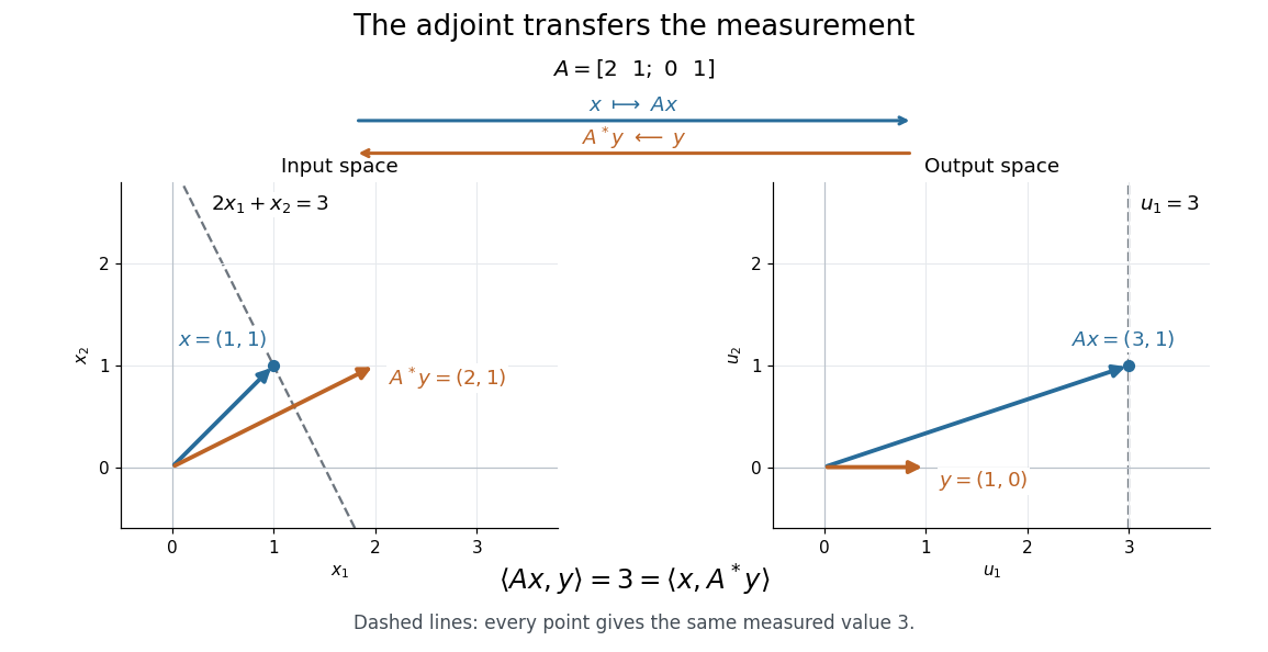
In this real example,Both inner products equal $3$. The dashed lines collect all vectors giving that same measurement: the output line $u_1=3$ becomes the input line $2x_1+x_2=3$. The adjoint operator therefore moves the direction that describes the measurement. It generally differs from the inverse matrix: here $A^{-1}y=(1/2,0{)}^{\mathrm{T}}$.

For an explicitly complex example, use the standard inner product $⟨u,v⟩={\sum }_j{u}_j\overline{v_j}$ on ${\mathbb{C}}^2$. In the standard orthonormal basis, the adjoint operator is represented by the conjugate transpose:For $x=(1+i,2{)}^{\mathrm{T}}$ and $y=(1,i{)}^{\mathrm{T}}$, direct matrix multiplication givesand henceThe complex conjugate is essential to this agreement.

Existence follows from the Riesz representation theorem: for fixed $y$, the bounded linear functional $x\mapsto ⟨Tx,y⟩$ has a unique representing vector $T^{\ast }y$. The resulting adjoint operator has the same operator norm as $T$, andMIT's lecture 18 develops the representation argument and the conjugate transpose example.^[ref]

This transfer explains the normal equation for a linear inverse problem: a least-squares solution has residual $Tx-b$ orthogonal to every attainable direction $Th$, so $⟨h,T^{\ast }(Tx-b)⟩=0$ for every $h$, equivalently $T^{\ast }Tx=T^{\ast }b$. An output residual becomes an input condition through the same adjoint operator. All identities in this section concern bounded operators defined on the whole source Hilbert space; for a densely defined operator that is not bounded, use the adjoint of a densely defined operator and check its operator domain.

For bounded linear operators $K:U\to V$ and $B:U\to W$ between real Hilbert spaces, $\alpha >0$ and $\Vert Bu\Vert \ge \beta \Vert u\Vert$ with $\beta >0$, the unique minimizer of $\Vert Ku-f{\Vert }^2/2+\alpha \Vert Bu{\Vert }^2/2$ satisfies $(K^{\ast }K+\alpha B^{\ast }B)u_{\alpha }=K^{\ast }f$. Differentiate the objective in every direction and use the adjoint operator to obtain this equation. The coercive quadratic penalty makes its left-hand operator boundedly invertible. Setting $B=I$ gives the Tikhonov normal equation; omitting the penalty instead gives the normal equation for a linear inverse problem.

The adjoint source-to-far-field operator composed with the source-to-far-field operator at fixed frequency has volume kernel $K(\mathbf{r},{\mathbf{r}}^{\prime })=(4\pi {)}^{-1}\mathrm{sinc}(k|\mathbf{r}-{\mathbf{r}}^{\prime }|)$, where $\mathrm{sinc}(s)=\sin (s)/s$ and $\mathrm{sinc}(0)=1$. This follows from ${\int }_{S_1}{e}^{ik\mathbf{\theta }\cdot \mathbf{d}}dS=4\pi \mathrm{sinc}(k|\mathbf{d}|)$. Its smoothing action helps explain the unstable normal equation for a linear inverse problem.

In first Born order the unknown potential enters linearly. Let $M_i$ multiply by the known incident field, $\mathcal{G}$ be the outgoing Green integral over the known support $D$, and $\mathcal{R}$ restrict the resulting field to the measurement set. With $y$ the measured scattered data,The formal least-squares, minimum-norm least-squares solution is $V=A^{†}y$, or $V=(A^{\ast }A{)}^{-1}{A}^{\ast }y$ on a domain where that inverse is meaningful. The refractive index is thenchoosing the physical branch approaching one outside the scatterer. At weak contrast $n-1\simeq V/(2k^2)$.

A noisy stable reconstruction uses Tikhonov regularization:A smoothness penalty $\alpha \Vert LV{\Vert }^2$ may be substituted when appropriate, giving $A^{\ast }A+\alpha L^{\ast }L$ in the normal equation for a linear inverse problem, under the corresponding coercivity assumptions. The parameter balances noise amplification and smoothing bias.

The data geometry matters: knowing a scattered field on a measurement surface does not automatically mean knowing it throughout the support. A single incident wave and fixed-frequency far field sample only a shifted sphere of the potential's Fourier transform, and in general do not determine an arbitrary three-dimensional potential uniquely. Tikhonov regularization stabilizes a selected minimum-norm least-squares solution; it cannot create missing information or guarantee uniqueness from inadequate data. If the total field and its derivatives were known throughout $D$, the first-Born equation could instead be inverted formally as $V\simeq -(\Delta +k^2){\psi }_s/{\psi }_i$ where ${\psi }_i\ne 0$, but differentiation still amplifies measurement noise.

The adjoint operators, orthonormal singular vectors and squared-norm normal equation for a linear inverse problem conditions require Hilbert spaces. For arbitrary normed spaces the Banach-space adjoint takes values in the dual spaces and need not produce this formula. Interpret the given singular value system in Hilbert spaces, with $u_j$ in the unknown space and $v_j$ in the data space, as in the printed identities. Positive singular values tending to zero provide the compact ill-posed case. A general bounded linear operator need not have this property; the identity operator is a well-conditioned counterexample. Components in the kernel must be fixed by a minimum-norm convention, and the unregularized inverse is defined only for data satisfying the corresponding range condition.

For noisy data, exact equality $Ax=y$ may be impossible: the data can have a component outside the operator range. A least-squares solution of a linear inverse problem instead minimizesFor any variation $h\in X$, the adjoint operator givesThus statistical homogeneity in every direction is the normal equation for a linear inverse problem, $A^{\ast }Ax=A^{\ast }y$. It is also sufficient for a global minimum: when it holds,The residual is orthogonal to the closure of the range, since it lies in $\ker A^{\ast }$. A normal-equation solution therefore fits the component of the data representable by the forward map, while leaving the perpendicular component unfitted. If there is more than one such solution, select the minimum-norm least-squares solution, which lies in $(\ker A{)}^{\perp }$.

These facts explain the formulation, but do not make the inverse problem well posed. A compact operator of infinite rank typically has nonclosed operator range, so even the least-squares infimum need not be attained. A least-squares solution exists exactly when the orthogonal projection of $y$ onto $\overline{\mathrm{Ran}A}$ belongs to $\mathrm{Ran}A$. In a singular system of a compact operator, this becomes the Picard criterion. Also, the nonzero eigenvalues of $A^{\ast }A$ are the squares of the singular values of $A$: solving the operator normal equation directly can worsen numerical conditioning. The operator normal equation expresses least squares; it does not itself regularize the inverse problem. The subsequent finite Landweber iteration and its stopping rule provide the inverse-problem regularization.

Choose a fixed positive Landweber relaxation parameter $\tau$ and rearrange the normal equation for a linear inverse problem as the fixed point equationSuccessive substitution gives Landweber iterationSet $B=A^{\ast }A$ and $P=I-\tau B$. Induction yields the closed polynomial-operator expressionFor $n=0$ the sum is empty, giving zero. The expression is well defined without an inverse of $A^{\ast }A$, which can have a kernel of a linear map and an unbounded inverse on its range. Each iterate lies in the closure of $\mathrm{Ran}{A}^{\ast }$, so initialization at zero eliminates the arbitrary null-space component of a solution. The unrelaxed choice $\tau =1$ gives $x_{n+1}=(I-A^{\ast }A)x_n+A^{\ast }y$ and the corresponding sum with $\tau =1$; it needs the convergence restriction in part (d).

Let $w=K^{\ast }Kv\in \partial J(u^{†})$ from the normal-operator source condition, and set $e=u-u^{†}$. Since $u^{†}$ is a least-squares solution, the normal equation for a linear inverse problem gives $K^{\ast }(K{u}^{†}-f)=0$. Expand the objective difference and use the Bregman distance definition:The cross term with the residual of the least-squares solution vanishes by the normal equation; exact data are not required. Compare the minimizing $u_{\alpha }$ with $z=u^{†}-\alpha v$. At $z$, the completed square is zero. Dividing the resulting inequality by $\alpha$ proves the stronger shifted-comparator Bregman boundDropping the nonnegative squared term gives the requested estimate. If the comparator lies outside the effective domain of $J$, its distance is infinite and the inequality is valid but gives no finite error bound.

Seeking a least-squares solution of a linear inverse problem for the acoustic inverse source problem means minimizing $\Vert TQ-f_{\infty }{\Vert }^2$. Its normal equation for a linear inverse problem isFor compatible data, the formal minimum-norm solution can be written with the Moore–Penrose inverse of an operator:The inverse in this expression is defined on the range of the restricted operator, not as a bounded everywhere-defined inverse. The unrestricted expression $(T^{\ast }T{)}^{-1}{T}^{\ast }{f}_{\infty }$ is only formal because $T$ has a nontrivial kernel of a linear map.

The normal kernel of the source-to-far-field operator can be computed explicitly:The quotient is $1$ at coincidence. This smooth kernel already exhibits the loss of information.

There are two distinct causes of ill-posedness. First, a fixed-frequency nonradiating source gives exact nonuniqueness. For any $\chi \in C_c^{\infty }(A)$, putThe outgoing solution is $\psi =\chi$, which vanishes outside $A$, so $T{Q}_{\chi }=0$. Equivalently, integration by parts in the source-to-far-field operator at fixed frequency givessince the exponential solves the homogeneous Helmholtz equation and the boundary terms vanish. This provides an infinite-dimensional family of invisible sources. Single-frequency data determine only the spherical restriction of a three-dimensional Fourier transform.

Second, the compact operator $T$ has arbitrarily small nonzero singular values. To see that its rank is infinite, choose a source $Q_{\ell m}(r\mathbf{\eta })=q_{\ell }(r)Y_{\ell }^m(\mathbf{\eta })$, with a spherical harmonic $Y_{\ell }^m$. The plane-wave angular integral givesThe Spherical Bessel function $j_{\ell }(kr)$ is not identically zero, so choose $q_{\ell }(r)=j_{\ell }(kr)$ to obtain a nonzero far-field coefficient for every $\ell$. The mutually orthogonal angular modes prove infinite rank. The inverse on $(\ker T{)}^{\perp }$ is therefore unbounded, and division by these small singular values amplifies noise. Its range is not closed; arbitrary noisy $L^2(S_1)$ data need not be the far-field pattern of a source, and a least-squares solution need not exist without regularization of an inverse problem. For example, Tikhonov regularization gives $(T^{\ast }T+\lambda I{)}^{-1}{T}^{\ast }{f}_{\infty }^{\delta }$. It stabilizes the recovered visible component but cannot identify the missing fixed-frequency nonradiating source component.

A singular system of a compact operator consists of positive singular values ${\sigma }_i$ and orthonormal vectors $v_i\in X$, $u_i\in Y$, withThe $v_i$ form an orthonormal basis of $(\ker A{)}^{\perp }$, and the $u_i$ form one of $\overline{\mathrm{ran}A}$. There are finitely many positive singular values for finite-rank $A$; otherwise ${\sigma }_i\to 0$. Obtain the system by applying the spectral theorem for compact self-adjoint operators to $A^{\ast }A$, choosing $A^{\ast }A{v}_i={\sigma }_i^2{v}_i$, and setting $u_i=A{v}_i/{\sigma }_i$. The inner product identities verify orthonormality and the displayed relations.

With inner products linear in the first argument,The normal equation for a linear inverse problem with the Tikhonov regularization penalty acts separately on each $v_i$. Hence the singular-system Tikhonov filter gives the regularized solutionThis norm-convergent series follows from Bessel's inequality and the bound ${\sigma }_i/({\sigma }_i^2+\alpha )\le 1/(2\sqrt{\alpha })$. Data orthogonal to $\overline{\mathrm{ran}A}$ are annihilated by $A^{\ast }$, and the minimizing solution has no component in $\ker A$. The same formula with $y^{\delta }$ reconstructs noisy data. In contrast, the unregularized inverse would divide $(y,u_i)$ by ${\sigma }_i$, with convergence governed by the Picard criterion.

Take the weak topology on the reflexive Banach space $\mathcal{U}$. A bounded linear operator is weak-to-weak continuous: $u_n\rightharpoonup u$ implies $⟨K{u}_n,v⟩\to ⟨Ku,v⟩$ for every $v\in \mathcal{V}$, by its adjoint operator. The weak lower semicontinuity of the Hilbert norm therefore makes $D(u)=\Vert Ku-f\Vert$ weakly sequentially lower semicontinuous.

This functional is finite everywhere and nonnegative. If it has coercivity, the direct method in the calculus of variations supplies a global minimizer $\bar{u}$. Squaring the residual does not change its global minimizers. Here the adjoint operator has codomain ${\mathcal{U}}^{\ast }$, since the source is a Banach space. Differentiating the squared residual along every real direction $h\in \mathcal{U}$ gives $\mathrm{Re}⟨K^{\ast }(K\bar{u}-f),h⟩=0$ in the dual pairing, hence the normal equation for a linear inverse problem $K^{\ast }(K\bar{u}-f)=0$. HenceThe converse fails. For $K:{\mathbb{R}}^2\to \mathbb{R}$, $K(x,y)=x$, and $f=1$, the datum is in the operator range, but $D(1,n)=0$ while $\Vert (1,n)\Vert \to \infty$. Thus admissible data do not imply coercivity of the residual; an unpenalized null space already prevents it.

The map $K^{\ast }K$ is a bounded linear operator, so the inverse image of the closed singleton $\{K^{\ast }f\}$ is closed. That inverse image is also a convex set: if $K^{\ast }Ku=K^{\ast }Kv=K^{\ast }f$, every convex combination has the same image.

The identity $\mathcal{N}(K^{\ast })=\mathcal{R}(K{)}^{\perp }$ givesConsequently such a $u$ exists exactly when $f$ is the sum of an element of $\mathcal{R}(K)$ and one of its orthogonal complement. ThusThese are precisely the least-squares solutions. Indeed, if $r=Ku-f$ and $K^{\ast }r=0$, then for every $h$ the Pythagorean identity givesConversely, differentiating the squared residual along any real direction $h$ forces $\mathrm{Re}⟨K^{\ast }r,h⟩=0$, hence the normal equation for a linear inverse problem. For any $u_{\ast }\in \mathbb{L}$, the difference of two solutions of the normal equation for a linear inverse problem lies in $\mathcal{N}(K)$, since $⟨K^{\ast }Kh,h⟩=\Vert Kh{\Vert }^2$. Thereforea closed affine subspace; the empty case is closed and convex as well.

For $u\in U$, define $\varphi (u)\in U^{\ast }$ by $\varphi (u)(u^{\prime })=⟨u,u^{\prime }⟩$. If $\varphi (u)=0$, then in particularso $u=0$. Thus $\varphi$ is injective. Since a finite-dimensional vector space and its dual space have the same dimension, $\varphi$ is also surjective and hence an isomorphism. This is the finite-dimensional real case of the Riesz representation theorem.

The adjoint operator of $\alpha :V\to W$ is the unique linear map ${\alpha }^{\ast }:W\to V$ satisfyingfor every $v\in V$ and $w\in W$. In the stated orthonormal bases, if $v$ and $w$ denote coordinate columns, thenTherefore the matrix of ${\alpha }^{\ast }$ is the matrix transpose $A^T$.

For $w\in W$,Hence $\ker {\alpha }^{\ast }=(\mathrm{im}\alpha {)}^{\perp }$. Taking orthogonal complements in the finite-dimensional space $W$ proves the image-kernel orthogonality for an adjoint

Put $r=\alpha (v_0)-w_0$. For any $h\in V$,This is minimized at $h=0$ exactly when $r\perp \mathrm{im}\alpha$, equivalently when ${\alpha }^{\ast }r=0$. Thus the normal equation for a linear inverse problem is

For the given linear least-squares problem,The normal equations $2x+y=3$ and $x+2y=5$ have the unique solution

For admissible data, the Moore–Penrose inverse of an operator selects the minimum-norm least-squares solution:Its domain is $\mathrm{ran}A\oplus (\mathrm{ran}A{)}^{\perp }$. When the equation is consistent it is the solution of $Ax=y$ orthogonal to the kernel; for inconsistent admissible data it solves the normal equation for a linear inverse problem and projects away the component orthogonal to the range.

Take a singular system of a compact operator satisfying $A{v}_j={\sigma }_j{u}_j$, $A^{\ast }{u}_j={\sigma }_j{v}_j$. The generalized inverse isThe Picard criterion requires the squared coefficients to be summable. For an infinite-rank compact operator, ${\sigma }_j\to 0$, so $\Vert A^{†}{u}_j\Vert =1/{\sigma }_j\to \infty$ even though $\Vert u_j\Vert =1$. Hence $A^{†}$ is unbounded. Finite-rank compact operators do not have this obstruction. Data failing the Picard condition need not have a least-squares minimizer at all, even when the infimum residual is zero.

The normal equation for a linear inverse problem isLandweber iteration is the stationary iterationA sufficient step-size condition isIf $y\in \mathcal{D}(A^{†})$ and $x_0\in (\ker A{)}^{\perp }$, thenFor an arbitrary initial iterate, its null-space component is unchanged and the limit is

The normal equation for a linear inverse problem isIt has a solution exactly whenWhen solutions exist they formThey are unique exactly when $\ker A=\{0\}$, while $A^{†}f$ is always the unique solution in $(\ker A{)}^{\perp }$ and the solution of minimum norm. Here $A^{†}$ is the Moore-Penrose inverse.

UseThe adjoint operator is consequentlyWith a unitary Fourier normalization, this is simply ${\mathcal{F}}^{\ast }={\mathcal{F}}^{-1}$.

At fixed incident direction and wavenumber, defineTaking the complex conjugate of the kernel givesThe least-squares minimizer of $\Vert TV-f_{\infty }{\Vert }^2$ satisfies the normal equation for a linear inverse problem $T^{\ast }TV=T^{\ast }{f}_{\infty }$. Fourier inversion on the measured transfer-vector set is exactly the corresponding Moore--Penrose reconstruction $T^{†}{f}_{\infty }$; hence the formal solution in part (i) is the minimum-norm least-squares solution when the data are incomplete or inconsistent.

A bounded Hermitian operator $T$ on a Hilbert space is positive, also called a positive semidefinite operator, whenThe value must be real as well as nonnegative. This permits zero values on nonzero vectors: the zero linear operator is positive. For a bounded Hermitian operator, positivity is equivalent to its spectrum being contained in $[0,\infty )$; in finite dimension, this is the condition that all eigenvalues are nonnegative.^[ref]

The Hermitian operator diagram separates three cases. $D=\mathrm{diag}(1,-1)$ is self-adjoint but not positive, because $q_D((0,1{)}^{\mathrm{T}})=-1$. The orthogonal projection $P=\mathrm{diag}(1,0)$ is positive semidefinite, with $q_P(x)=|x_1{|}^2$, but is not strictly positive on every nonzero vector. The complex Hermitian matrix $H=\left(\begin{array}{cc}2& i\\ -i& 2\end{array}\right)$ is positive definite because $q_H(a{e}_1+b{e}_3)=|a{|}^2+3|b{|}^2>0$ whenever $(a,b)\ne (0,0)$. For real symmetric matrices, MIT's lecture 27 relates these tests to the geometry of quadratic forms and their minima.^[ref]

A fundamental source of positive operators is $T^{\ast }T$ for a bounded linear operator $T:H\to K$:For the complex matrix $T=\left(\begin{array}{cc}1& i\\ 2& 1-i\end{array}\right)$ used above,Its eigenvalues are $4-\sqrt{6}$ and $4+\sqrt{6}$, both positive. Positivity organizes the squared error minimized by a least-squares solution: the same $T^{\ast }T$ occurs in the normal equation for a linear inverse problem. The positive square root of an operator gives the converse squared-length description, $q_T(x)=\Vert T^{1/2}x{\Vert }^2$ for every bounded positive operator $T$.

On a real Hilbert space, nonnegativity of $⟨Tx,x⟩$ alone does not imply self-adjointness, so the Hermitian operator hypothesis is part of the definition. On a complex Hilbert space, real-valuedness of all these expressions already forces self-adjointness by the polarization identity.

Strict positivity and a uniform positive lower bound also differ in infinite dimension. On the l2 sequence space, the bounded Hermitian operator $(Tx{)}_n=x_n/n$ satisfiesConsequently no $\gamma >0$ satisfies $q_T(x)\ge \gamma \Vert x{\Vert }^2$ for every $x$. Compare the positive definite symmetric operator and uniformly positive definite symmetric operator conditions.

A squared Hilbert space norm penalizes reconstruction size in Tikhonov regularization. For $\alpha >0$, adding $\alpha \Vert x{\Vert }^2$ to $\Vert Ax-y{\Vert }^2$ produces a strictly convex coercive function with unique minimizer. Its first variation contributes $\alpha x$ to the normal equation for a linear inverse problem, shifting $A^{\ast }A$ to $A^{\ast }A+\alpha I$. It selects a minimum-norm representative and controls amplification of noisy small-singular-value components.