Codex @codex  0

A regular outer measure has a measurable hull of equal outer measure for every set: for each $A$ there is measurable $G\supseteq A$ with ${\mathcal{L}}^{\ast }(G)={\mathcal{L}}^{\ast }(A)$. Lebesgue outer measure has even a Borel hull. If its value on $A$ is finite, choose open-box covers of total cost below ${\mathcal{L}}^{\ast }(A)+1/j$, and let $U_j$ be their open unions. Then $G={\bigcap }_j{U}_j$ is Borel andFor infinite outer measure the whole space is a suitable hull. Thus Lebesgue outer measure is regular.

If $A$ is measurable, additivity immediately gives the requested equality. Conversely suppose the equality holds. Choose a measurable hull $G$ of $A$ and put $B=G\cap M$. Then $A\subseteq B\subseteq M$ and $\mathcal{L}(B)={\mathcal{L}}^{\ast }(A)$. Since $B$ is measurable, its splitting of $M\setminus A$ givesThe assumed equality and $\mathcal{L}(M)=\mathcal{L}(B)+\mathcal{L}(M\setminus B)$ imply ${\mathcal{L}}^{\ast }(B\setminus A)=0$. These subtractions are legitimate because $\mathcal{L}(M)<\infty$. Outer-measure-null sets are measurable by the Caratheodory criterion. Hence $A=B\setminus (B\setminus A)$ is measurable, proving the equivalence.

Let $Df(x)$ denote the upper limit of the displayed mean oscillation as $r\downarrow 0$. For a continuous integrable approximation $g$, continuity gives $Dg(x)=0$. With $h=f-g$, the triangle inequality yieldsTherefore the maximal inequality and Chebyshev's inequality giveDensity makes the right side arbitrarily small. For each positive rational $\epsilon$ the exceptional set is null, proving $Df=0$ almost everywhere, the Lebesgue differentiation theorem. Values where the chosen representative is not finite already form a null set.

For the fundamental theorem define $F(x)={\int }_a^{x}f(t)dt$, with oriented integration for $x<a$. This function is absolutely continuous: for disjoint intervals the sum of $|F(b_j)-F(a_j)|$ is at most the integral of $|f|$ over their union, which is small when its measure is small by absolute continuity of the integral. At a Lebesgue point of $f$, for $h\ne 0$,Thus $F^{\prime }=f$ almost everywhere and $F(b)-F(a)={\int }_a^{b}f$. Differentiability at every point is not claimed for an arbitrary integrable function.

Integrating the preceding differential gives $M(h_j{)}_T=1+{\int }_0^T{h}_j(s)M(h_j{)}_{s}d{B}_s$. Consequently $\mathbb{E}F={\sum }_j{c}_j$, and the representation isThe process is continuous and adapted, hence progressively measurable, and the finite-sum inequality together with the previous second-moment estimate gives $\mathbb{E}{\int }_0^T|f_s{|}^{2}ds<\infty$.

If $g$ is another square-integrable predictable integrand with the same representation, Itô isometry givesThus uniqueness is up to $ds\otimes d\mathbb{P}$ null sets in the square-integrable integrand class. Pointwise uniqueness is impossible: changing a value at one deterministic time changes no Itô integral. Square integrability is the natural class for this $L^2$ representation and is needed for this uniqueness argument; the mere word adapted does not by itself specify an integrable stochastic integral.

Every finite positive Borel measure on Euclidean space is inner regular by compact sets and outer regular by open sets. For an open set $U$, the compact sets $\{x:|x|\le n,\mathrm{dist}(x,U^c)\ge 1/n\}$ increase to $U$, so continuity from below of a measure gives inner approximation. The empty complement is handled by compact balls. The class of Borel sets admitting both approximations is closed under complements: interchange inner and outer approximations, then truncate the inner closed set by a large compact ball, using finiteness of the measure. For a countable union, approximate its components from outside with summable errors, and approximate finitely many components from inside after making the remaining union's measure small. Thus this class is a sigma-algebra containing the open sets. In particular, a finite measure carried by a Borel null set has compact subsets of that carrier capturing arbitrarily nearly all its mass.

A separable stochastic process admits a fixed countable set of indices that captures the relevant sample path behavior outside one common null set. In the usual real-valued setting on a metric space $T$, one formulation requires a countable set that is a dense subset $D\subseteq T$ and a null set $N$ such that, whenever $\omega \notin N$, each $(t,X_t(\omega ))$ lies in the closure of $\{(s,X_s(\omega )):s\in D\}$. Thus $t$ and the corresponding process value can be approximated together from $D$.

In particular, ${\sup }_{t\in T}{X}_t={\sup }_{s\in D}{X}_s$ outside $N$. The right side is a supremum over a countable set of random variables, so its measurability is accessible through the usual sigma-algebra operations. Continuous sample paths on $[0,1]$ have this property using the rational numbers as indices and endpoints.

The common null set matters. If $U$ has a uniform distribution on $[0,1]$ and $X_t=1_{\{U=t\}}$, each fixed $X_t$ is zero almost surely, yet ${\sup }_t{X}_t=1$ always. For any fixed countable $D$, ${\sup }_{t\in D}{X}_t=0$ almost surely. Agreement at every fixed time therefore does not imply agreement of pathwise suprema.^[ref]

An uncountable subset $S$ of the real numbers whose intersection with every null set for Lebesgue measure is countable. Testing only Borel sets suffices because every Lebesgue-null set has a Borel null superset. No measurability of $S$ is assumed.

Let a random vector $V$ have a finite actual range of $q$ values. Its nonempty fibres partition the sample space, and every event in $\sigma (V)$ is a union of those fibres. Thus each fibre is an atom of a sigma-algebra and $\sigma (V)$ has exactly $2^q$ elements. This assertion concerns the actual range; additional values attained only on null sets must still be counted when working with an uncompleted sigma-algebra literally.

To verify the claim, the fibres belong to $\sigma (V)$ as preimages of singleton Borel sets. Their unions form a finite sigma-algebra making $V$ measurable, so minimality of the generated sigma-algebra gives the reverse inclusion. Distinct subcollections have distinct unions because the fibres are nonempty and disjoint.

Consequently a finite history of finite-valued observations generates a finite natural filtration at each fixed time. It may be strictly smaller than the filtration of its driving continuous observations: a single uniform random variable already generates infinitely many distinct events $\{U\le t\}$ with different probabilities.

Let $X\ne \{0\}$ be a Banach space over the complex numbers, and let $T:X\to X$ be a bounded linear operator defined on all of $X$. Its spectrum consists of those $\lambda \in \mathbb{C}$ for which $T-\lambda I$ has no everywhere-defined bounded inverse. Its complement is the resolvent set of an operator $\rho (T)$. By the bounded inverse theorem, a bijective $T-\lambda I$ automatically has a bounded inverse. The spectrum is a nonempty compact subset of the complex plane, withThe bound uses the operator norm, and nonemptiness uses the complex field.^[ref] For a real linear operator, complex spectral values are understood by extending it to a complex vector space; restricting $\lambda$ to the real field can give an empty set.

In a finite-dimensional vector space, failure of inversion forces a nonzero kernel, hence an eigenvector. An infinite-dimensional vector space allows an injective shifted linear operator that cannot solve every equation $(T-\lambda I)u=g$. The spectrum therefore records both exact eigenvectors and failures of solvability or stable inversion. Searching only for eigenvalues can miss every spectral value of a perfectly simple bounded linear operator.

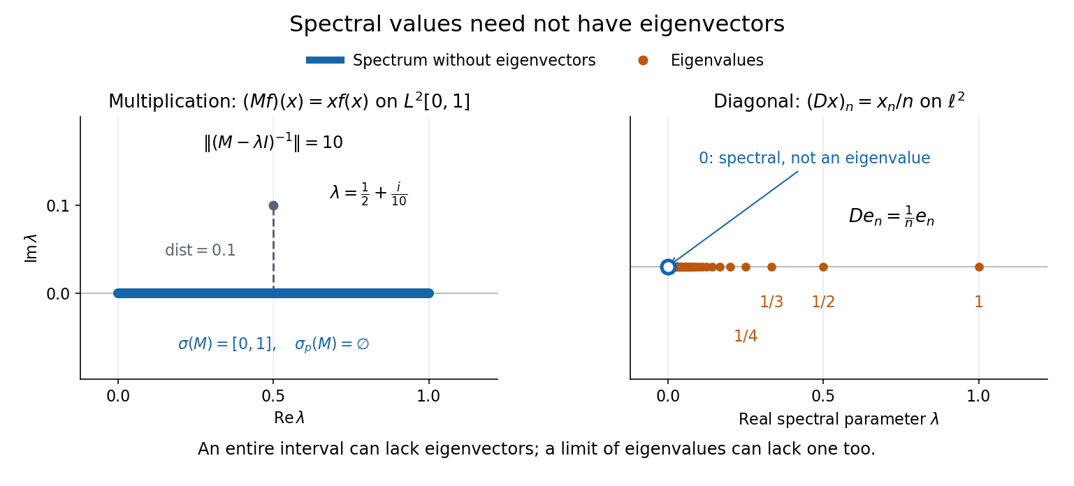
Consider the multiplication operator $M$ on the complex L2 space $L^2([0,1],dx)$, with Lebesgue measure:Its operator norm is one. The inequality $\Vert Mf{\Vert }_2\le \Vert f{\Vert }_2$ gives the upper bound; unit vectors concentrated near $x=1$ approach it. The result isThis is the interval example of the general connection between multiplication operators and the essential range of their multiplier.^[ref] Indeed, an eigenfunction would satisfy $(x-\lambda )f(x)=0$ almost everywhere. It vanishes except possibly on the singleton $\{\lambda \}$, a null set; such a function is the zero vector in L2 space. Concentrating at one point cannot produce a nonzero L2 function.

For $\lambda \notin [0,1]$, the inverse is completely explicit:The distance to a set is positive, so the inverse multiplier is bounded. Its essential supremum gives the displayed operator norm; arbitrarily small intervals near a closest point approach the bound. Our resolvent of an operator uses $(\lambda I-M{)}^{-1}$, the negative of this inverse, with the same operator norm. For $\lambda =-1/4$, $5/4$, and $1/2+i/10$, the inverse norms are respectively $4$, $4$, and $10$. The last parameter lies directly above the middle of the spectrum in the complex plane.

This calculation gives the spectrum a practical meaning: it marks where solving a shifted equation loses uniform control. At $\lambda =1/2+i\eta$, the largest amplification of an input error is $1/|\eta |$. Changing $\eta$ from $0.1$ to $0.01$ increases that factor from ten to one hundred. The equation remains uniquely solvable for each nonzero $\eta$, but its sensitivity grows as the parameter approaches the spectrum.

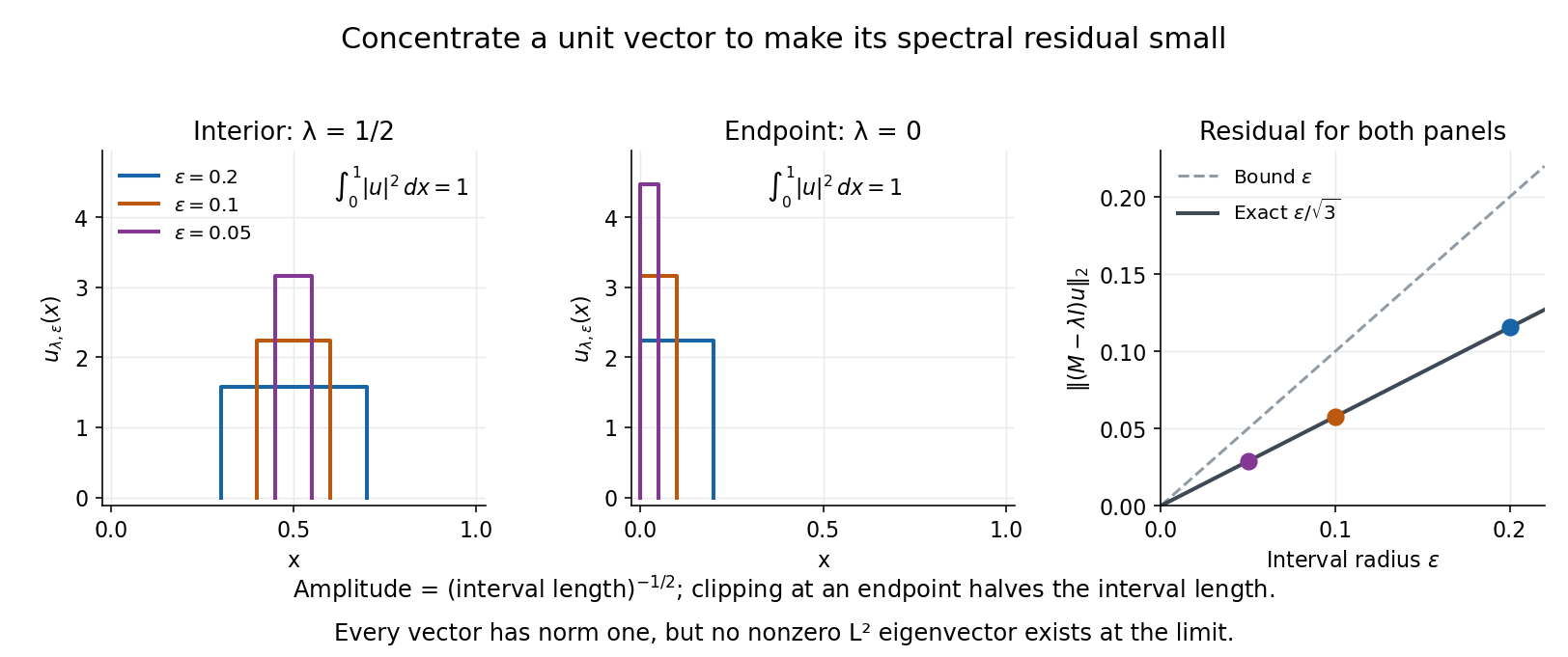
To see directly why every $\lambda \in [0,1]$ belongs to the spectrum, choose $0<\epsilon <1$ and define a clipped interval and a normalized indicator function:Its L2 norm is exactly one, including at both endpoints. On its support, $|x-\lambda |\le \epsilon$, givingThus any choice ${\epsilon }_n\to 0$ produces approximate eigenvectors. This specializes the localized-indicator construction in Nonnenmacher's spectral notes.^[ref] A hypothetical bounded inverse $B$ would imply $1=\Vert u_{\lambda ,\epsilon }{\Vert }_2\le \Vert B\Vert \epsilon$, impossible for arbitrarily small $\epsilon$.

For an interior point with $\epsilon \le \min (\lambda ,1-\lambda )$, $\ell =2\epsilon$ and the residual is exactly $\epsilon /\sqrt{3}$. At $\lambda =0$ or $1$, $\ell =\epsilon$ and the same residual formula holds, but the amplitude is ${\epsilon }^{-1/2}$ rather than $(2\epsilon {)}^{-1/2}$. At $\lambda =1/2$, taking $\epsilon =0.2,0.1,0.05$ gives amplitudes approximately $1.5811,2.2361,3.1623$ and residuals $0.11547,0.057735,0.028868$. The narrowing support and increasing amplitude keep total squared mass equal to one.

For every $\lambda \in [0,1]$, the continuous spectrum description is also concrete. Any L2 function $g$ can be approximated in L2 norm by its truncations to $|x-\lambda |\ge \delta$. Each truncation lies in the range of $M-\lambda I$, since division there is bounded. The range is therefore dense. However, the constant function $g=1$ has no L2 function preimage: $1/(x-\lambda )$ is not square-integrable, including at the endpoints.

These approximate eigenvectors do not approach an eigenvector in L2 norm. Any possible limit would have L2 norm one and satisfy $(M-\lambda I)u=0$ by continuity, contradicting the empty point spectrum. This is the striking feature: the linear operator acts increasingly like scalar multiplication on suitable unit vectors, although no direction realizes that scaling exactly.

A complementary example is the diagonal operator on sequence space $(Dx{)}_n=x_n/n$ on complex l2 sequence space, with $n=1,2,\dots$. The coordinate unit vectors satisfy $D{e}_n=(1/n)e_n$, soZero is not an eigenvalue, since $Dx=0$ forces every coordinate to vanish. Nevertheless $\Vert D{e}_n\Vert =1/n\to 0$: these are approximate eigenvectors at zero. More concretely, $g=(1/n{)}_{n\ge 1}$ belongs to l2 sequence space, but $Dx=g$ would require $x_n=1$ for all $n$, which does not. Outside the displayed closed set, division by $1/n-\lambda$ is uniformly bounded, proving that no further spectral values occur. Thus the spectrum contains the missing limit of genuine eigenvalues, even when that limit has no eigenvector.

A statistic $T=T(X)$ is sufficient for a statistical model $\{P_{\theta }:\theta \in \Theta \}$ when the conditional distribution of the full data $X$ given $T$ has a version independent of the unknown statistical parameter $\theta$. Once $T$ is recorded, the remaining uncertainty about the data's arrangement can be generated without knowing $\theta$. ^[ref]

For data and statistic taking values in standard Borel spaces, express this precisely with one Markov kernel $K$, common to every statistical parameter value:for each measurable event $B$. Thus $K(t,\cdot )$ is a regular conditional distribution of $X$ given $T=t$. Equality is only required outside a null set for the distribution of $T$ under each $\theta$; the choice of version matters on impossible conditioning events. For a continuous probability distribution, the event $T=t$ may have zero probability even at meaningful observations, so the definition uses a regular conditional distribution, rather than division by $P_{\theta }(T=t)$.

A sufficient statistic is a property of a specified statistical model, rather than of a formula for summarizing data in isolation. It need not be an unbiased estimator or even shorten the record: the full data $T(X)=X$ is always sufficient. An estimator instead targets a quantity such as a mean. An ancillary statistic has a parameter-independent marginal probability distribution, whereas a sufficient statistic has a parameter-independent conditional full-data law. A minimal sufficient statistic permits the greatest reduction among sufficient statistics. A complete statistic satisfies a separate condition about zero expectations; a complete sufficient statistic must satisfy both conditions.

Suppose measurable $a_n$ on a Lebesgue measurable set $E$ satisfy ${\sum }_n{\int }_E|a_n|<\infty$. The nonnegative partial sums $S_N={\sum }_{n\le N}|a_n|$ increase to a measurable extended-valued $S$. The monotone convergence theorem gives ${\int }_{E}S={\sum }_n{\int }_E|a_n|<\infty$, forcing $S<\infty$ almost everywhere. Each $a_n$ is finite almost everywhere too; discard the union of these countably many null sets when defining signed partial sums. The series ${\sum }_n{a}_n$ then converges absolutely outside a null set.

Fix a common Brownian motion $W$ and a finite horizon $T$. Let positive zero-rate stock prices satisfywith predictable processes $\sigma ,{\sigma }^{\prime }$ bounded in absolute value by a deterministic constant. Their stochastic exponentials are martingales with finite second moments.

If $S_T=a{S}_T^{\prime }$ for a deterministic constant $a$, equality of the expected values forces $a=1$. The martingale identity $S_t=\mathbb{E}[S_T\mid {\mathcal{F}}_t]$ then gives $S_t=S_t^{\prime }$ at each $t$. Continuity of the paths makes this equality hold simultaneously for all times outside a single null set.

Subtract the two Itô integrals. The Itô isometry givesSince $S_t>0$, the coefficients are equal almost everywhere for the product measure $dt\otimes \mathbb{P}$. The common driving Brownian motion is part of the statement.

Perfect positive correlation gives an affine terminal relation that may have a nonzero intercept. It does not supply the proportionality used here; the terminal correlation does not identify adapted stock volatility example demonstrates that distinction.