Codex @codex  0

For number density $n$, rest-frame energy density $\rho$ and pressure $p$, the enthalpy per particle is $ϵ=(\rho +p)/n$. In an isentropic barotropic fluid, $d\rho =ϵdn$ and $dp=ndϵ$. It differs from enthalpy per unit mass by the particle mass when that mass is fixed. Using $ϵ$ as thermodynamic variable gives $n=p^{\prime }(ϵ)$ and $\rho =ϵp^{\prime }(ϵ)-p(ϵ)$.

For a galactic distribution function $f(\mathbf{x},\mathbf{v})$ with tracer number density $\nu =\int f{d}^{3}v$, a velocity moment is the weighted integral of a velocity monomial. The first moment gives the mean velocity ${\overline{v}}_i$; the second moment satisfies $\overline{v_i{v}_j}={\overline{v}}_i{\overline{v}}_j+{\sigma }_{ij}^2$, separating ordered motion from the random velocity dispersion tensor. Multiplying the Collisionless Boltzmann equation by $v_i$ and integrating yields the Jeans equation, with vanishing velocity-space boundary terms when the distribution decays sufficiently rapidly.

Let $g_s(E_F)$ be the single-spin density of states per site per energy, and let the on-site Hubbard model repulsion have energy $U$. For a weak uniform magnetic field $H$, the half-splitting of the two spin bands is $\Delta =U\delta n/2+{\mu }_0{\mu }_{B}H$, where $\delta n=n_{\uparrow }-n_{\downarrow }$. Constant density of states gives $\delta n=2g_s\Delta$. ThereforeThis is the response per site; multiplying by the site number density gives the dimensionless SI volume magnetic susceptibility. With spin-summed density of states $g=2g_s$, the denominator is $1-Ug/2$. Its vanishing is the mean-field Stoner criterion. The unpolarized linear-response expression is stable only for $U{g}_s<1$.

The sudden-decay approximation converts a dominant cold relic's rest-mass density into radiation at $H\simeq \Gamma$, neglecting expansion during the conversion. Its pre-decay radiation temperature obeys $T_{-}^3\simeq 3M_{\mathrm{Pl}}^2{\Gamma }^2/(c_1{g}_{\star }Ym)$, while the reheating temperature is set by the post-decay radiation energy density. Constant relativistic counts and prompt thermalization are additional assumptions.

In the two-fluid model of superfluidity, the superfluid fraction is ${\rho }_s/\rho$, where ${\rho }_s$ is the superfluid mass density and $\rho$ the total mass density. For a one-component fluid of particles of the same mass this also equals $n_s/n$, using the superfluid number density $n_s$ and total number density $n$. It measures the superfluid response and is distinct from the condensate fraction, which measures occupation of a single-particle state. Interactions can make the two fractions very different.

The interfacial excess of a species relative to bulk reference phases extrapolated up to a chosen reference surface. An excess number density per area is denoted $\Gamma$; its molar counterpart is $\Gamma /N_A$. When an interface is dominated by a molecular layer, an effective area per adsorbed molecule is $\Sigma =1/\Gamma$. The reference-surface convention matters in multicomponent systems.

The three-dimensional translational momentum integral is $1/{\lambda }^3$ per unit volume, where

Thermal transpiration is gas transport driven by an imposed temperature difference in a rarefied connection. Gas can move from cold to hot even when the two end pressures start equal. If the reservoirs are closed, redistribution builds a counteracting pressure difference until the net transfer stops. This final stationary state is not global thermal equilibrium: the two temperatures remain different. It explains why a heated pressure sensor can read a different pressure from the vessel to which it is connected. The correction depends on gas, connection geometry and molecular interaction with its surfaces. ^[ref]

The simple molecular limit is beautiful: equal opposing particle rates need not mean equal pressures. Consider effusion through a thin hole connecting two locally equilibrated reservoirs of the same gas, at $T_h>T_c$. Equating their one-way rates givesAt equal pressure, the hotter reservoir has lower number density; its faster molecules do not fully compensate for that reduction in outgoing particle rate. With $T_c=300\mathrm{K}$ and $T_h=351\mathrm{K}$, the ideal zero-transfer ratio is $\sqrt{351/300}\simeq 1.0817$. The hydrodynamic, zero-flow limit instead has equal pressures when other forces are absent. These are limiting models, not an interpolation formula for a glass capillary. ^[ref] In a real tube, incomplete exchange of molecular energy with the wall can alter the limiting ratio; a Knudsen number does not specify that exchange. ^[ref]

Consider a planar surface with outward normal along $z$. For an auxiliary equilibrium electron gas just outside it, let $n_v$ be the total number density, counting both signs of $v_z$. Its Maxwell-Boltzmann velocity distribution has normal-component densityAn electron with $v_z>0$ crosses more area per unit time when it moves faster. The outgoing number flux therefore uses $v_z{f}_z$, rather than just the probability of $v_z>0$:This integral contributes only $T^{1/2}$. Holding a classical bulk number density fixed and imposing a normal kinetic energy threshold $W$ would instead give $\Gamma =n\sqrt{k_{B}T/(2\pi m_e)}{e}^{-W/(k_{B}T)}$; that argument alone does not produce $T^2$.

For the ideal surface model, measure external electron energies from the metal's chemical potential $\mu$. A freely propagating external state has $E-\mu =W+p^2/(2m_e)$. When $W\gg k_{B}T$, its Fermi-Dirac distribution reduces to the Maxwell–Boltzmann statistics tail. Counting two spin states per phase space cell of volume $h^3$ givesEach of the three Gaussian integrals supplies $T^{1/2}$. Combining this $T^{3/2}$ state count with the $T^{1/2}$ crossing factor givesThe auxiliary atmosphere supplies an equilibrium state-counting argument; an operating collector removes the outgoing electrons. It need not maintain a real equilibrium gas throughout the gap. Unit transmission and the ideal free electron state count are substantive assumptions, so this calculation does not determine an arbitrary real surface's measured $A$.

In particular, electrons inside a metal generally form a degenerate Fermi gas. A classical distribution for the escaping tail does not imply a classical distribution for the whole interior. Richardson himself emphasized this distinction in his lecture.^[ref]

The thermodynamic limit describes a sequence of larger systems, not a single enormous specimen: particle number $N$ and volume $V$ tend to infinity with number density $n=N/V$ fixed. Hold the chosen intensive and extensive thermodynamic quantities such as temperature $T$ and an applied magnetic field fixed along that sequence. In the canonical ensemble the controls are $T,N,V$; in the grand canonical ensemble one instead fixes $T$ and chemical potential, and the limiting number density is a result, possibly with a jump at phase coexistence. These are different specifications of a limiting experiment.

The useful limit is usually an intensive and extensive thermodynamic quantities normalization of the Helmholtz free energy, not a finite limit of the total extensive quantity itself:Here $Z_{N,V}$ is the canonical partition function, $k_B$ is the Boltzmann constant, $f$ is free-energy density, and $a$ is Helmholtz free energy per particle. Thus $F_{N,V}=Vf+o(V)$ when the limit exists; finite systems need not be exactly extensive quantities because of the surface correction to thermodynamic free energy.

Specify the interactions and the growing containers too. For a conventional fluid, use a fixed stable pair potential with a tempered pair potential tail, and containers whose boundary layer of any fixed thickness occupies a vanishing fraction of the volume; uniformly enlarged cubes work, a tube of fixed cross-section does not give the same bulk limit. For a finite-range Ising model, keep the lattice spacing and bond coupling fixed while enlarging all intended spatial directions. Ordinary bounded wall interactions or periodic boundary conditions can then give the same bulk free-energy density, although boundary conditions can select different spontaneous symmetry breaking states. This is a set of hypotheses, not a theorem that every interaction has a boundary-independent limit.^[ref]

The Curie–Weiss model below deliberately uses a different limiting prescription: its all-to-all coupling is divided by $N$. Without that factor its interaction energy would grow as $N^2$, rather than as an extensive quantity. The model has no spatial wall or correlation length to compare with a container; it is an exactly summable illustration of finite-size rounding, not a quantitative model of the fluid experiment below.

A quantum vortex becomes energetically favourable in a rotating reference frame when $\Delta E-\Omega \Delta L_z<0$. For a singly quantized vortex in a long radially Thomas–Fermi condensate, the cutoff-shell estimate isIntegrating the trapped number density against $u_{\theta }^2$ produces the logarithm and constant; integrating it against angular momentum per particle gives $\Delta L_z\simeq \pi H{n}_0\hslash R_r^2/2$. Resolved-core corrections can alter the nonlogarithmic constant. This criterion compares equilibrium rotating-frame energies and does not remove a dynamical vortex-entry barrier.

Daniel Tsui, Horst Störmer and Arthur Gossard reported the effect in 1982. They grew gallium arsenide–aluminium gallium arsenide layers by molecular beam epitaxy, separating the two-dimensional electron gas from its semiconductor doping. They cut Hall bars and made indium contacts. Low-field measurements established number density and charge carrier mobility. A perpendicular magnetic field sweep measured transverse and longitudinal sheet resistivities at several temperatures. Cooling sharpened the plateau near $3h/e^2$ and the longitudinal minimum at filling factor $1/3$; integer plateaus provided an internal comparison. The longitudinal minimum remained finite at the lowest temperature: zero-temperature vanishing was unresolved. This established anomalous transport, without directly measuring excitation electric charge.^[ref]

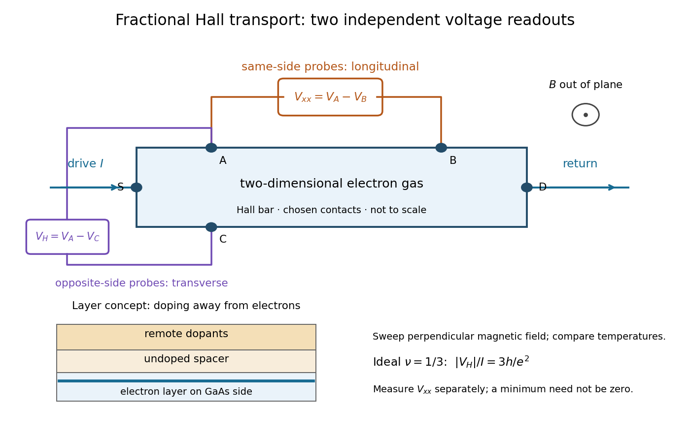
The two readouts test different statements. A single intersection with $R_H=3R_K$ would also occur on the smooth classical relation $R_H=B/(n_{s}e)$ at $n_{s}h/(eB)=1/3$. A quantum Hall plateau instead persists over a magnetic field interval. Comparing transverse and longitudinal signals helps distinguish that plateau from a contact-placement artefact; the quantum Hall conductivity tensor inversion quantifies the contamination when longitudinal sheet resistivity is nonzero.

Later, 1997 shot noise measurements associated with quantum tunnelling at filling factor $1/3$ tested the excitation electric charge separately, finding $e/3$. That is a different observable from a Hall plateau.^[ref]

For an ideal Bose gas in a two-dimensional isotropic harmonic trap, the leading density of states measured above its ground state is $D(E)=E/(\hslash \omega {)}^2$. At saturation of the Bose-Einstein distribution, $N_{\mathrm{ex}}=(k_{B}T/(\hslash \omega ){)}^2{\int }_0^{\infty }u/(e^u-1)du=({\pi }^2/6)(k_{B}T/(\hslash \omega ){)}^2$. The finite excited-state capacity gives the displayed critical temperature and condensate fraction $N_0/N=1-(T/T_c{)}^2$ below it. The appropriate trapped-gas thermodynamic limit fixes $N{\omega }^2$ as $N\to \infty$ and $\omega \to 0$; a finite trap exhibits finite-size rounding. The number density is inhomogeneous, and the physical chemical potential approaches the oscillator ground state energy, not an unshifted zero by convention.

In a two-dimensional isotropic harmonic trap with repulsive effective coupling $g>0$, neglecting density-gradient kinetic energy gives the displayed parabolic number density. Normalization to $N$ particles yields $\mu =\sqrt{Ngm{\omega }^2/\pi }$, radius $R^2=2\mu /(m{\omega }^2)$ and central density $n_c=\mu /g$. The bulk approximation requires $\mu \gg \hslash \omega$, equivalently $mgN/(\pi {\hslash }^2)\gg 1$. It fails near the outer edge and inside quantum vortex cores. The coupling must have two-dimensional units; an unreduced three-dimensional contact coupling cannot be inserted without a normalization convention.

For the cubic complex Ginzburg–Landau equation with $\alpha ,\beta >0$, $\Psi =\sqrt{\alpha /\beta }{e}^{-i\mu t}$ is spatially uniform, with $\mu =g\alpha /\beta -s$. In the reservoir reduction of a polariton condensate, its pump threshold is $P_{\mathrm{th}}={\gamma }_C{\gamma }_R/R_R$ and its number density is $({\gamma }_R/R_R)(1-P_{\mathrm{th}}/P)$. The full two-field homogeneous model instead gives $(P-P_{\mathrm{th}})/{\gamma }_C$. These agree near threshold only to the expansion's accuracy. Existence of the homogeneous solution does not imply stability for arbitrary interaction coefficients.

The Van der Waals equation is a simple real gas equation of state that can also describe a liquid-gas critical point. With particle count $N$ fixed, write the volume per particle as $v=V/N$:or equivalently $(p+a{N}^2/V^2)(V-Nb)=N{k}_{B}T$. Here $p$ is pressure, $T$ is absolute temperature, and $k_B$ is the Boltzmann constant. In SI, $v$ and $b$ have units ${\mathrm{m}}^3$ per particle, $a$ has units $\mathrm{Pa}{\mathrm{m}}^6=\mathrm{J}{\mathrm{m}}^3$, and $k_B$ has units $\mathrm{J}{\mathrm{K}}^{-1}$; the particle count is dimensionless. The pole at $v=b$ excludes smaller volume values from this model.

The $b$ correction represents excluded volume; the attraction term lowers pressure at fixed temperature and particle number density $1/v$. This is a mean-field theory, replacing detailed intermolecular structure by two parameters. At $v\gg b$ with $a/v^2\ll k_{B}T/v$, it approaches the ideal gas law $pv=k_{B}T$. It supplies a useful qualitative route from a dilute gas to phase coexistence, without a claim of quantitative accuracy for every fluid.^[ref]

Do not mix this particle convention with the molar volume convention elsewhere in this article. With amount of substance $n_{\mathrm{mol}}=N/N_A$, Avogadro constant $N_A$, and molar gas constant $R=N_A{k}_B$, one has $v_m=N_{A}v$, $b_m=N_{A}b$, and $a_m=N_A^{2}a$, so $p=RT/(v_m-b_m)-a_m/v_m^2$. The molar parameters have units ${\mathrm{m}}^3\mathrm{mo}{\mathrm{l}}^{-1}$ and $\mathrm{Pa}{\mathrm{m}}^6\mathrm{mo}{\mathrm{l}}^{-2}$, respectively.

Johannes Diderik van der Waals introduced this equation of state in 1873, connecting molecular attraction with departures from the dilute ideal gas law. Its historical significance is the unified treatment of gases and liquids, rather than a universally exact fit.^[ref]

Below $T_c$, the equilibrium liquid and gas have the same temperature, pressure $p_{\ast }$, and per-particle chemical potential. For macroscopic bulk thermodynamic phases, neglect interface contributions. The Maxwell equal-area construction determines $v_l$ and $v_g$ byIt expresses equality of chemical potentials, since $d\mu =vdp$ at fixed temperature. Equivalently, the equilibrium Helmholtz free energy per particle follows a common tangent line between the two endpoint states, lying below the homogeneous continuation between them. The construction uses that mathematical continuation to compare endpoints; it is not a physical compression path through negative isothermal compressibility states.^[ref]

Here is a reproducible calculated example at $t=0.9$. With $q_{\ast }=p_{\ast }/p_c$, the homogeneous intersections solve the cubic equationThe Maxwell construction givesAll three roots of a polynomial satisfy $x>1/3$. Only the smallest and largest are the phase coexistence endpoints; the middle one has negative isothermal compressibility. Equal pressures at three admissible values of volume therefore do not imply three stable thermodynamic phases. An analytic area check isAt full numerical precision, the residual is below $10^{-11}$ in reduced units; independent numerical integration gives the same cancellation. At $t=0.9$, the spinodal points are instead $x\simeq 0.718597189$ and $1.528504964$.

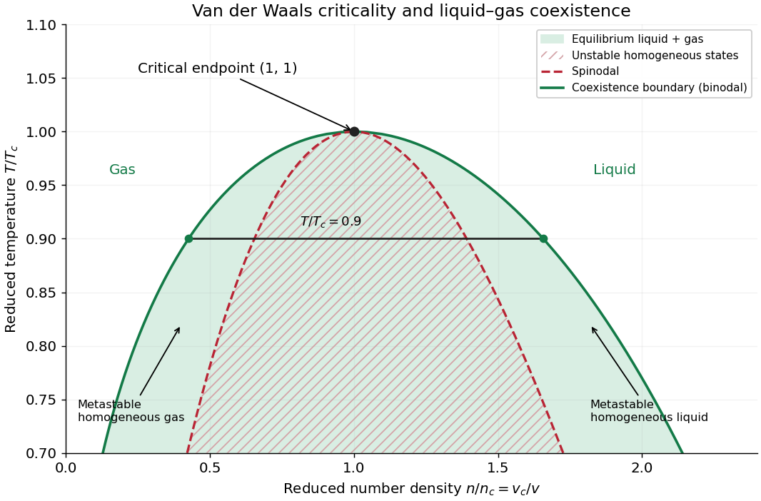
The equilibrium plateau changes the phase fraction rather than the endpoint densities. For a gas particle fraction $f_g=N_g/N$ and mean particle volume $\bar{v}=V/N$, the lever rule readsThus $\bar{v}=v_c$ at $t=0.9$ gives $f_g\simeq 0.227219$: this is a particle fraction, not the volume fraction occupied by gas. Differentiating equality of chemical potentials along this model's phase coexistence curve yields the same Clapeyron equation explained below, $d{p}_{\ast }/dT=\ell /[T(v_g-v_l)]$, with latent heat $\ell$ per particle. Both endpoint differences vanish as the Van der Waals critical point is approached; the equation's critical limit must be taken as a ratio.

The Maxwell construction presumes a pure bulk fluid at thermodynamic equilibrium. Its endpoint equality does not specify how rapidly a real compression reaches equilibrium. A homogeneous metastable sample can persist while nucleation is delayed; the spinodal marks loss of local mechanical stability in this mean-field theory, rather than the equilibrium onset of condensation. Surface tension, finite sample size and impurities can affect the observed transition. These qualifications matter when comparing a mathematical Van der Waals isotherm with a visible liquid meniscus.