Use the source's Gaussian units and neglect the displacement current, as in nonrelativistic magnetohydrodynamics. Write for the pressure anisotropy. The pressure tensor is , so its force density isAmpère's law and the solenoidal magnetic-field constraint give the Lorentz force decompositionAdding these two force densities and using yieldsThe first term is the gradient of the modified magnetohydrodynamic total pressure; the second is the anisotropic Maxwell stress tensor contribution together with the directional pressure force. Their effective coefficient is the pressure-anisotropy-modified magnetic tension, . At fixed magnetic field, positive pressure anisotropy increases resistance to bending, while negative pressure anisotropy reduces it. When becomes negative, bending experiences an amplifying force rather than a restoring force. Gradients of can also drive motion, so the curvature interpretation refers specifically to the bending contribution.
Set and . Distinguish the scalar magnetic field strength perturbation from the vector perturbation . To first order,where the last identity is the solenoidal magnetic-field constraint. For a Fourier mode with the stated time convention, putThe linear momentum conservation equation, after division by , isUse the solenoidal magnetic-field constraint in its component. The coefficient of reduces to . ThusBoth scalar pressure perturbations act within the plane. The component therefore decouples, independently of their closure. The ideal magnetohydrodynamic equations giveEliminating the amplitudes gives the Alfvén wave dispersion relationFor this Shear Alfvén wave, the velocity and fluid displacement are along , perpendicular to both and the equilibrium magnetic field. Let ; thenA real snapshot bends the magnetic field lines sideways, with . There is no first-order compression or change of magnetic field strength: , and . Scalar pressure perturbations are unnecessary in this transverse subsystem. For a traveling stable branch, , so the velocity and transverse magnetic field perturbations are in phase or opposite phase according to the branch. At the bending force and this angular frequency vanish.
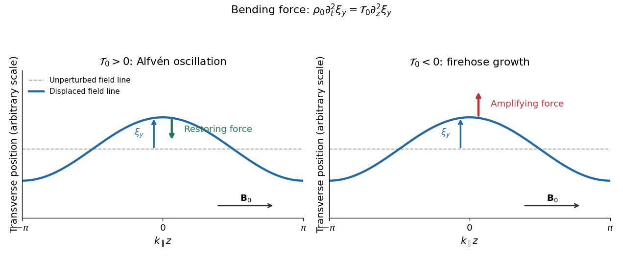

For the Alfvén wave becomes a firehose instability when its squared angular frequency is negative:Equality is marginal, rather than exponential growth. The pressure anisotropy must have negative sign; its absolute magnitude alone is insufficient.
For the intergalactic plasma, a negative relative pressure anisotropy of reaches this fluid threshold only for . In particular, the literal pair and relative pressure anisotropy is stable because the threshold is . Since the quoted numbers are approximate and allow larger plasma beta, this weakly magnetized plasma is susceptible, rather than necessarily unstable at every quoted value. For example, and relative pressure anisotropy are unstable. Positive pressure anisotropy does not excite this branch.
For the fusion-device plasma, requires a negative relative pressure anisotropy below roughly , whereas its magnitude is only about . The stabilizing magnetic tension dominates, so it is not susceptible to this fluid firehose instability under the stated conditions. Indeed, nonnegative perpendicular pressure requires the relative pressure anisotropy to be no smaller than ; at such a small plasma beta even this extreme cannot satisfy the threshold.
Magnetic flux freezing ties a transverse fluid displacement to a bend in the magnetic field lines. For the uniform background, the transverse displacement equation isFor a sinusoidal bend, . Positive pressure-anisotropy-modified magnetic tension therefore gives a restoring force, and inertia produces oscillation. In an isotropic plasma, this is precisely the positive magnetic tension .
Particles moving predominantly along bent magnetic field lines contribute a transverse momentum flux. Their larger parallel pressure opposes the restoring curvature force supplied by the magnetic field and perpendicular pressure. Once , the net force points along the original displacement: a larger bend produces a larger outward force, giving positive feedback. Equivalently, the bending contribution to the quadratic potential energy is and has become negative.
In this static, homogeneous fluid model the unstable roots areWith the root grows. Its real angular frequency is zero, so the unstable pattern grows without propagation in the equilibrium rest frame; its partner decays. Advection by a background flow would change that frame-dependent statement. The growth increasing without bound as increases is a limitation of this long-wavelength model: finite gyroradius and other kinetic corrections cannot be neglected at sufficiently short scales.
Label a trajectory by and write its flow map as , with . An infinitesimal material line joining neighboring labels has tangent , where is the deformation gradient. Differentiating at fixed labels givesThis identity holds for an unnormalized material line tangent even in a compressible flow. Incompressibility also makes an advected magnetic field obey the same stretching law. A unit tangent would instead require a projection removing its change of length.
Use the source's velocity gradient convention . For a outer product , the product rule yieldsThe same law holds for a sum or locally transported average of such outer products. Thus the dyadic transport of material line elements motivatesThis upper-convected derivative vanishes for a symmetric tensor transported solely by stretching of material lines. It subtracts both advection and geometric deformation, allowing a constitutive equation to isolate intrinsic relaxation or production. More generally gives . Under a time-dependent rigid rotation , its value transforms as , making it an objective time derivative. This is a suitable derivative for this transport type; symmetry alone does not make it the unique possible objective time derivative.
When deformation is stopped, the rate-of-strain tensor and velocity gradient vanish, leaving . HenceThe positive constant is the viscoelastic relaxation time. For slow weak deformation, all the transport and quadratic terms are smaller than , so . Thus is the zero-rate dynamic viscosity, measured in stress times time. The corresponding short-time shear modulus of the Maxwell fluid response is . The source's has units of time, since must have units of stress.
Linearize about a relaxed state with constant mass density . In the unforced momentum conservation equation , the component of the pressure gradient is zero for a freely evolving unidirectional flow independent of . A prescribed external pressure gradient would add a forcing term.
For , incompressibility is automatic and the only nonzero entries of the rate-of-strain tensor are . Products of stress and velocity gradient are quadratic in the small amplitude. The constitutive equation consequently becomes to first order. With , its shear component and the component of momentum conservation areThe diagonal stress components have only homogeneous relaxation at this order and vanish if initially relaxed. In particular, does not enter this linear response.
Eliminating the shear stress from the two linear equations gives the Maxwell shear-wave dispersion equation in physical space,where is the kinematic viscosity. Substitution of a Fourier mode givesThese are temporal exponents: the oscillation angular frequency is the imaginary part of , with the sign determined by the selected time convention. For both exponents are real and nonpositive. At equality the repeated exponent is ; generic solutions include . Above the threshold the modes are damped propagating shear disturbances:At large their phase velocity tends to .
For the limit at fixed and , expansion of the square root givesAfter a short initial relaxation, the surviving branch obeys the diffusion equation of a Newtonian fluid. The fast branch disappears on the vanishing viscoelastic relaxation time; at the two exponents are exactly and . This limit is not uniform in : modes with of order still sample the oscillatory transition. If instead is held fixed as , then and the fixed- slow exponent tends to zero. The ordinary Newtonian fluid limit therefore specifies which material parameter is held fixed.
Let and use for the source's velocity gradient convention. Seek the homogeneous stationary stress reached under steady simple shear flow. The material derivative of that stress tensor vanishes. In the plane,The , and components of the constitutive equation give, respectively,Thus, putting and using the shear stress calculated below,The out-of-plane shear components vanish on the homogeneous branch. The two normal-stress differences areThe ratio is defined at nonzero shear when ; at both differences vanish, and the displayed constant is their limiting ratio. An arbitrary isotropic pressure in the total Cauchy stress tensor cancels from both differences; it is not an arbitrary addition to the constitutively defined extra stress itself.
The component of the stationary constitutive equation isInsert and . The coefficient of becomes , givingFor , the small-rate shear stress is . At large positive rate, and the shear viscosity decreases as . The shear stress is odd in rate, reaches a positive maximum atand decreases thereafter. The original plot displays this homogeneous constitutive curve. Its decreasing branch can permit shear banding; the local model alone supplies neither an interface-selection rule nor a guaranteed stable homogeneous realization.
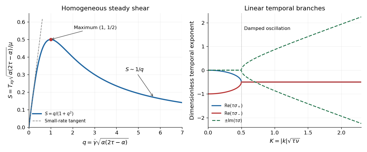
Homogeneous shear stress and the two temporal branches of the linear response
. The steady curve uses q equal to the shear rate times the square root of alpha times (2 tau minus alpha). The spectral panel uses K equal to the wavenumber magnitude times the square root of tau times nu. These are distinct nondimensional variables. Details.
This is a Johnson-Segalman fluid without an added Newtonian fluid solvent contribution. To identify conventions explicitly, set and , with the spin tensor. The derivative appearing in the constitutive equation becomesthe Gordon--Schowalter derivative. Its usual slip interval corresponds to , while a nonsingular genuinely shear thinning curve requiresAt the model is the Upper-convected Maxwell model; at it is the lower-convected derivative counterpart, and both have constant shear viscosity in this test. At the derivative is the Jaumann derivative, giving the corotational Maxwell fluid. Merely requiring is insufficient: for the denominator is , which vanishes at and then gives a negative steady shear viscosity. There is no solvent-induced large-rate plateau in the stated equation.
Articles by others on the same topic
There are currently no matching articles.